Scaling Sensors with Data Synthesis
120 likes | 246 Vues
In an era where data availability is unprecedented, the challenge lies in making sense of vast information generated by advanced sensor technologies. This work explores innovative strategies to navigate and understand environmental data in real-time. By employing a synthesis approach that combines observation, analysis, and validation, researchers can better predict ecological changes across various scales. The role of sensors, data analysis, and public policy is examined, highlighting the implications for biofuels and climate studies, while emphasizing the need for interdisciplinary methods to address complex environmental challenges.

Scaling Sensors with Data Synthesis
E N D
Presentation Transcript
Scaling Sensors with Data Synthesis Catharine van Ingen eScience Group Microsoft Research It was six* men of Indostan, to learning much inclined,Who went to see the elephant though all of them were blind, That each by observation, might satisfy his mind. *data reporting error
Unprecedented Data Availability • Created by the confluence of fast internet connectivity, commodity computing and advanced sensor technologies • Ever more pressing challenge is how to make sense of it all
Navigatingin Real-Timeand Real-Space Globe 107 m Evolution 109 y Continent 106 m Speciation, Extinction 106 y • Challenge: How do we use data to think about the future when the past is no longer a good predictor? • Strategy: Scale up and down to bridge understanding and observational capabilities • Approach: {mashup, derive, validate, analyze} repeat • Hope: There are some technologies and methodologies that generalize to other disciplines with time and space drivers Landscape 103 - 105 m Species migration, Soil formation 103 y Canopy 100 - 103 m Succession, Mortality 102 y Plant 10-1 - 100 m Competition, Gap Creation 101 y Leaf 10-2 – 10-1 m Stomata 10-5 m Crop cycles 100 y Sensors are the ante; Synthesis is the game Chloroplast 10-6 m Photosynthesis 10-6 -10-3 y
Data-Driven Science Meets Public Policy and Economics • GPP, or gross photosynthetic production is component of carbon fixation and tied to water balance • Implications for biofuels – GPP is higher in southern temperate forests than in the mid-west Corn Belt Thanks to Dennis Baldocchiand Youngryel Ryu (UC Berkeley) 2010
About That Map • Existing upscalingmethods leverage sensor categorical aggregates • Black(ish) box statistics applied to land cover informed by modeled or remote sensed meteorology • Parameterization for biophysical model synthesis computation • Simulation is not an option • Radiative transfer meets turbulence meet ssystem biology • Existing climate models “do not evince much skill” at capturing the biological processes • Science disclaimer: Biofuel is more complex • Efficient and renewable biofuel production includes factors such as harvest efficiency and transportation costs
Penman-Monteith (1964) Theory Meets Reality • Big reduction : many inputs • Not a matrix : some inputs have geospatial categorical dependencies ET= Water volume evapotranspired (m3 s-1 m-2) Δ = Change rate of sat. specific humidity with air temp.(Pa K-1) λv = Latent heat of vaporization (J/g) Rn = Net radiation (W m-2) cp = Specific heat capacity of air (J kg-1 K-1) ρa = dry air density (kg m-3) δq = vapor pressure deficit (Pa) ra = Resistance of air (m s-1) rs = Resistance of plant stoma, air (m s-1) γ = Psychrometric constant (γ ≈ 66 Pa K-1) Estimating resistance across a catchment can be tricky
Heterogeneous Data Sources forestinventoryplot century Forest/soil inventories decade Landsurface remote sensing Eddycovariancesensor towers Talltower sensorobser- vatories Remote sensingof CO2 year Temporal scale month week day hour local 0.1 1 10 100 1000 10 000 global Countries EU plot/site Spatial scale [km] Thanks to Markus Reichstein(Max Planck) 2010
Sourcing from Imagery, Sensors, Models, Field Data and Wisdom Climate classification ~1MB (1file) http://www.fluxdata.org FLUXNET curated sensor dataset 30GB (960 files) Vegetative clumping ~5MB (1file) FLUXNET curated fielddataset 2 KB (1 file) NASA MODIS imagery archives 5 TB (600K files) 10 US years 1 global year ~ 13 US years NCEP/NCAR ~100MB (4K files)
Validation Classic Local: direct pixel comparison with ground deployment • Known good or known bad Global: qualitative map views and large aggregates comparison • Includes inter-annual variations Radiation model expected to underestimate in the tropics Global GPP 118± 26 PgG/y literature range 107-167
Validation Vanguard The great frontier of unknown unknowns • Qualitative map observations require local knowledge – crowd source via citizen science? • Geospatial feature determination errors can be significant Shows high summer water use in the rice growing region of the Sacramento Valley and (blue) rock outcrop
Scaling: The Synthesis Trifecta • Science • Incorporate discovered or known omissions such as elevation, fires, storms, fertilizer • Regional analysis flame tests • Sensors • Refining existing sensors and variable derivations • Incorporating new emerging sensors such as web cams • Substrate • Move compute to data • Supercomputer size, but not supercomputing friendly • Data discovery, reuse, harmonization Sacramento Delta 10 year average evapotranspiration Phenocam detecting leaf green up and green down Sensors are ~20 KM apart – one shows impact of calibration drift
Anecdote, Analysis, Action I was walking Dry Creek and saw stranded fish… ..had local farmers turned on sprinklers? Flow vs Temperature 2008 Detail