More on Least Squares Fit (LSQF)
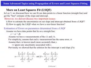
Some Advanced Topics using Propagation of Errors and Least Squares Fitting. More on Least Squares Fit (LSQF) In Lec 5, we discussed how we can fit our data points to a linear function (straight line) and get the "best" estimate of the slope and intercept.

More on Least Squares Fit (LSQF)
E N D
Presentation Transcript
Some Advanced Topics using Propagation of Errors and Least Squares Fitting More on Least Squares Fit (LSQF) In Lec 5, we discussed how we can fit our data points to a linear function (straight line) and get the "best" estimate of the slope and intercept. However, we did not discuss two important issues: I) How to estimate the uncertainties on our slope and intercept obtained from a LSQF? II) How to apply the LSQF when we have a non-linear function? Estimation of Errors on parameters determined from a LSQF Assume we have data points that lie on a straight line: y = a + bx Assume we have n measurements of the x’s and y's. For simplicity, assume that each y measurement has the same error, . Assume that xis known much more accurately than y. Þignore any uncertainty associated with x. Previously we showed that the solution for the intercept and slope is: P416/Lecture 7
Since and are functions of the measurements (yi's) we canuse the Propagation of Errors technique to estimate and . Assume that: a) Each measurement is independent of each other (sxy=0). b) We can neglect any error (s) associated with x. c) Each y measurement has the same s, i.e. si=s. See lecture 4 (general formula for 2 variables) assumption a) assumption b) assumption c) plugging our formula for a P416/Lecture 7
variance in the intercept We can find the variance in the slope () using exactly the same procedure: P416/Lecture 7
variance in the slope • n If we don't know the true value of , we can estimate the variance using the spread between the measurements (yi’s) and the fitted values of y: • n -2 = number of degree of freedom • = number of data points - number of parameters () extracted from the data • n If each yi measurement has a different error i: The above expressions simplify to the “equal variance” case. Don't forget to keep track of the “n’s” when factoring out equal ’s. For example: weighted slope and intercept P416/Lecture 7
Example: Fit to straight line 4 y 2 x 1 2 3 4 (same data as Lec 6) Previous fit to: f(x,b)=1+bx, b=1.05 New fit to: f(x,b)=a+bx, a =1.158±0.253 b=1.011± 0.072 a and b calculated using weighted fit (Taylor, P 198) χ2=0.65 for 2 degrees of freedom P(χ2>0.65 for 2dof) = 72% Errors on a and b calculated using: P416/Lecture 7
lLSQF with non-linear functions: u For our purposes, a non-linear function is a function where one or more of the parameters that we are trying to determine (e.g. , from the straight line fit) is raised to a power other than 1. n Example: functions that are non-linear in the parameter : However, these functions are linear in the parameters A. u The problem with most non-linear functions is that we cannot write down a solution for the parameters in a closed form using, for example, the techniques of linear algebra (i.e. matrices). n Usually non-linear problems are solved numerically using a computer. n Sometimes by a change of variable(s) we can turn a non-linear problem into a linear one. Example: take the natural log of both sides of the above exponential equation: lny=lnA-x/t=C+Dx Now a linear problem in the parameters C and D! In fact it’s just a straight line! To measure the lifetime (Lab 7) we first fit for D and then transform D into . u Example: Decay of a radioactive substance. Fit the following data to find N0 and : nN represents the amount of the substance present at time t. n N0 is the amount of the substance at the beginning of the experiment (t = 0). n is the lifetime of the substance. t = -1/D P416/Lecture 7
Lifetime Data n The intercept is given by: C = 4.77 = ln A or A = 117.9 ln[N(t)] time, t P416/Lecture 7
uExample: Find the values A and ttaking into account the uncertainties in the data points. • n The uncertainty in the number of radioactive decays is governed by Poisson statistics. • n The number of counts Ni in a bin is assumed to be the average (m) of a Poisson distribution: • m = Ni = Variance • n The variance of yi(= ln Ni) can be calculated using propagation of errors: • n The slope and intercept from a straight line fit that includes uncertainties in the data points: If all the s's are the same then the above expressions are identical to the unweighted case. a=4.725 and b = -0.00903 t= -1/b = -1/0.00903 = 110.7 sec n To calculate the error on the lifetime (t), we first must calculate the error on b: • The experimentally determined lifetime is: t= 110.7 ± 12.3 sec. Taylor P198 and problem 8.9 P416/Lecture 7
We can calculate the c2 to see how “good” the data fits an exponential decay distribution: Least Squares Fitting-Exponential Example For this problem: lnA=4.725 ®A=112.73 and t = 110.7 sec Poisson approximation Mathematica Calculation: Do[{csq=csq+(cnt[i]-a*Exp[-x[i]/tau])^2/(a*Exp[-x[i]/tau])},{i,1,10}] Print["The chi sq per dof is ",csq/8] xvt=1-CDF[ChiSquareDistribution[8],csq]; Print["The chi sq prob. is ",100*xvt,"%"] The chi sq per dof is 1.96 The chi sq prob. is 4.9 % This is not such a good fit since the probability is only ~4.9%. P416/Lecture 7
The Error on the Mean Error on the mean (review from Lecture 4) Question: If we have a set of measurements of the same quantity: What's the best way to combine these measurements? How to calculate the variance once we combine the measurements? Assuming Gaussian statistics, the Maximum Likelihood Method says combine the measurements as: If all the variances (s21= s22= s23..) are the same: The variance of the weighted average can be calculated using propagation of errors: weighted average unweighted average And the derivatives are: sx=error in the weighted mean P416/Lecture 7
If all the variances are the same: The error in the mean (sx) gets smaller as the number of measurements (n) increases. Don't confuse the error in the mean (sx) with the standard deviation of the distribution ()! If we make more measurements: The standard deviation (s) of the (gaussian) distribution remains the same, BUT the error in the mean (sx) decreases Lecture 4 Example: Two experiments measure the mass of the proton: Experiment 1 measures mp=950±25 MeV Experiment 2 measures mp=936±5 MeV Using just the average of the two experiments we find: mp=(950+936)/2=943MeV Using the weighted average of the two experiments we find: mp=(950/252+936/52)/(1/252 +1/52)=936.5MeV and the variance: s2=1/(1/252 +1/52)=24 MeV2 s=4.9 MeV Since experiment 2 was more precise than experiment 1 we would expect the final result to be closer to experiment 2’s value. mp=(936.5±4.9) MeV P416/Lecture 7