Decision Analysis
Chapter 3. Decision Analysis. Learning Objectives. List the steps of the decision-making process Describe the types of decision-making environments Make decisions under uncertainty Use probability values to make decisions under risk. After completing this chapter, students will be able to:.

Decision Analysis
E N D
Presentation Transcript
Chapter 3 Decision Analysis
Learning Objectives List the steps of the decision-making process Describe the types of decision-making environments Make decisions under uncertainty Use probability values to make decisions under risk After completing this chapter, students will be able to:
Learning Objectives Develop accurate and useful decision trees Revise probabilities using Bayesian analysis Use computers to solve basic decision-making problems Understand the importance and use of utility theory in decision making After completing this chapter, students will be able to:
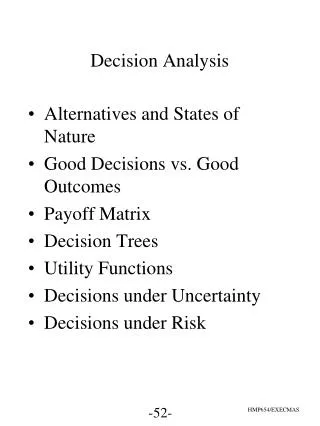
Chapter Outline 3.1 Introduction 3.2 The Six Steps in Decision Making 3.3 Types of Decision-Making Environments 3.4 Decision Making under Uncertainty 3.5 Decision Making under Risk 3.6 Decision Trees 3.7 How Probability Values Are Estimated by Bayesian Analysis 3.8 Utility Theory
Introduction What is involved in making a good decision? Decision theory is an analytic and systematic approach to the study of decision making A good decision is one that is based on logic, considers all available data and possible alternatives, and the quantitative approach described here
The Six Steps in Decision Making Clearly define the problem at hand List the possible alternatives Identify the possible outcomes or states of nature List the payoff or profit of each combination of alternatives and outcomes Select one of the mathematical decision theory models Apply the model and make your decision
Other Methods Non-quantitative methods Delphi Method Delphi – ‘the Oracle’ in ancient Greece that gave predictions about the future Finding a knowledgeable, wise person or persons to help make decisions In-house methods Executive Opinion/Decision Marketing Surveys
Thompson Lumber Company Step 1 – Define the problem • Expand by manufacturing and marketing a new product, backyard storage sheds Step 2 – List alternatives • Construct a large new plant • A small plant • No plant at all Step 3 – Identify possible outcomes • The market could be favorable or unfavorable
Thompson Lumber Company Step 4 – List the payoffs • Identify conditional values for the profits for large, small, and no plants for the two possible market conditions Step 5 – Select the decision model • Depends on the environment and amount of risk and uncertainty Step 6 – Apply the model to the data • Solution and analysis used to help the decision making
Thompson Lumber Company Table 3.1
Types of Decision-Making Environments Type 1: Decision making under certainty Decision maker knows with certainty the consequences of every alternative or decision choice Type 2: Decision making under uncertainty The decision maker does not know the probabilities of the various outcomes Type 3: Decision making under risk The decision maker knows the probabilities of the various outcomes
Decision Making Under Uncertainty Maximax (optimistic) Maximin (pessimistic) Criterion of realism (Hurwicz) Equally likely (Laplace) Minimax regret There are several criteria for making decisions under uncertainty
Maximax Maximax Used to find the alternative that maximizes the maximum payoff • Locate the maximum payoff for each alternative • Select the alternative with the maximum number Table 3.2
Maximin Maximin Used to find the alternative that maximizes the minimum payoff • Locate the minimum payoff for each alternative • Select the alternative with the maximum number Table 3.3
Criterion of Realism (Hurwicz) A weighted average compromise between optimistic and pessimistic • Select a coefficient of realism • Coefficient is between 0 and 1 • A value of 1 is 100% optimistic • Compute the weighted averages for each alternative • Select the alternative with the highest value Weighted average = (maximum in row) + (1 –)(minimum in row)
Criterion of Realism (Hurwicz) Realism • For the large plant alternative using = 0.8(0.8)(200,000) + (1 – 0.8)(–180,000) = 124,000 • For the small plant alternative using = 0.8 (0.8)(100,000) + (1 – 0.8)(–20,000) = 76,000 Table 3.4
Equally Likely (Laplace) Equally likely Considers all the payoffs for each alternative • Find the average payoff for each alternative • Select the alternative with the highest average Table 3.5
Minimax Regret Based on opportunity loss or regret, the difference between the optimal profit and actual payoff for a decision • Create an opportunity loss table by determining the opportunity loss for not choosing the best alternative • Opportunity loss is calculated by subtracting each payoff in the column from the best payoff in the column • Find the maximum opportunity loss for each alternative and pick the alternative with the minimum number
Minimax Regret • Opportunity Loss Tables Table 3.6 Table 3.7
Minimax Regret Minimax Table 3.8
Who Are You? Are you minimax regret? Are you maximax? A couple of points: When people are in different situations they can make decisions differently E.g., At work vs. at home As time goes on, a person may change in their attitude E.g., Old people are more conservative because they have no income and need to keep their money risk free.
Decision Making Under Risk • Decision making when there are several possible states of nature and we know the probabilities associated with each possible state • Most popular method is to choose the alternative with the highest expected monetary value (EMV) EMV (alternative i) = (payoff of first state of nature) x (probability of first state of nature) + (payoff of second state of nature) x (probability of second state of nature) + … + (payoff of last state of nature) x (probability of last state of nature)
EMV for Thompson Lumber • Each market has a probability of 0.50 • Which alternative would give the highest EMV? • The calculations are EMV (large plant) = (0.50)($200,000) + (0.50)(–$180,000) = $10,000 EMV (small plant) = (0.50)($100,000) + (0.50)(–$20,000) = $40,000 EMV (do nothing) = (0.50)($0) + (0.50)($0) = $0
EMV for Thompson Lumber Largest EMV Table 3.9
Expected Value of Perfect Information (EVPI) EVPI places an upper bound on what you should pay for additional information EVPI = EVwPI– Maximum EMV EVwPI is the long run average return if we have perfect information before a decision is made EVwPI = (best payoff for first state of nature) x (probability of first state of nature) + (best payoff for second state of nature) x (probability of second state of nature) + … + (best payoff for last state of nature) x (probability of last state of nature)
Expected Value of Perfect Information (EVPI) Scientific Marketing, Inc. offers analysis that will provide certainty about market conditions (favorable) Additional information will cost $65,000 Is it worth purchasing the information?
Expected Value of Perfect Information (EVPI) • Best alternative for favorable state of nature is build a large plant with a payoff of $200,000 Best alternative for unfavorable state of nature is to do nothing with a payoff of $0 EVwPI = ($200,000)(0.50) + ($0)(0.50) = $100,000 • The maximum EMV without additional information is $40,000 EVPI = EVwPI– Maximum EMV = $100,000 - $40,000 = $60,000
Expected Value of Perfect Information (EVPI) So the maximum Thompson should pay for the additional information is $60,000 • Best alternative for favorable state of nature is build a large plant with a payoff of $200,000 Best alternative for unfavorable state of nature is to do nothing with a payoff of $0 EVwPI = ($200,000)(0.50) + ($0)(0.50) = $100,000 • The maximum EMV without additional information is $40,000 EVPI = EVwPI– Maximum EMV = $100,000 - $40,000 = $60,000
Expected Opportunity Loss Expected opportunity loss (EOL) is the cost of not picking the best solution First construct an opportunity loss table For each alternative, multiply the opportunity loss by the probability of that loss for each possible outcome and add these together Minimum EOL will always result in the same decision as maximum EMV Minimum EOL will always equal EVPI
Expected Opportunity Loss Minimum EOL Table 3.10 EOL (large plant) = (0.50)($0) + (0.50)($180,000) = $90,000 EOL (small plant) = (0.50)($100,000) + (0.50)($20,000) = $60,000 EOL (do nothing) = (0.50)($200,000) + (0.50)($0) = $100,000
Sensitivity Analysis • Sensitivity analysis examines how our decision might change with different input data • For the Thompson Lumber example P = probability of a favorable market (1 – P) = probability of an unfavorable market
Sensitivity Analysis EMV(Large Plant) = $200,000P– $180,000)(1 – P) = $200,000P– $180,000 + $180,000P = $380,000P– $180,000 EMV(Small Plant) = $100,000P– $20,000)(1 – P) = $100,000P– $20,000 + $20,000P = $120,000P– $20,000 EMV(Do Nothing) = $0P + 0(1 – P) = $0
Sensitivity Analysis EMV Values $300,000 $200,000 $100,000 0 –$100,000 –$200,000 EMV (large plant) Point 2 EMV (small plant) Point 1 .167 .615 1 Values of P EMV (do nothing) Figure 3.1
Sensitivity Analysis Point 1: EMV(do nothing) = EMV(small plant) Point 2: EMV(small plant) = EMV(large plant)
Sensitivity Analysis EMV Values $300,000 $200,000 $100,000 0 –$100,000 –$200,000 EMV (large plant) Point 2 EMV (small plant) Point 1 EMV (do nothing) .167 .615 1 Values of P Figure 3.1
Using Excel QM to Solve Decision Theory Problems Program 3.1A
Using Excel QM to Solve Decision Theory Problems Program 3.1B
Decision Trees Any problem that can be presented in a decision table can also be graphically represented in a decision tree Decision trees are most beneficial when a sequence of decisions must be made All decision trees contain decision points or nodes and state-of-nature points or nodes A decision node from which one of several alternatives may be chosen A state-of-nature node out of which one state of nature will occur
Five Steps toDecision Tree Analysis Define the problem Structure or draw the decision tree Assign probabilities to the states of nature Estimate payoffs for each possible combination of alternatives and states of nature Solve the problem by computing expected monetary values (EMVs) for each state of nature node
Structure of Decision Trees Trees start from left to right Represent decisions and outcomes in sequential order Squares represent decision nodes Circles represent states of nature nodes Lines or branches connect the decisions nodes and the states of nature
Thompson’s Decision Tree A State-of-Nature Node Favorable Market A Decision Node 1 Unfavorable Market Construct Large Plant Favorable Market Construct Small Plant 2 Unfavorable Market Do Nothing Figure 3.2
Thompson’s Decision Tree EMV for Node 1 = $10,000 = (0.5)($200,000) + (0.5)(–$180,000) Payoffs (0.5) $200,000 Alternative with best EMV is selected (0.5) –$180,000 (0.5) $100,000 (0.5) –$20,000 = (0.5)($100,000) + (0.5)(–$20,000) EMV for Node 2 = $40,000 $0 Favorable Market 1 Unfavorable Market Construct Large Plant Favorable Market Construct Small Plant 2 Unfavorable Market Do Nothing Figure 3.3
Thompson’s Complex Decision Tree Payoffs First Decision Point Second Decision Point Favorable Market (0.78) $190,000 2 Unfavorable Market (0.22) Large Plant –$190,000 Favorable Market (0.78) Small Plant $90,000 3 Unfavorable Market (0.22) –$30,000 Survey (0.45) Results Favorable No Plant –$10,000 1 Favorable Market (0.27) $190,000 4 Unfavorable Market (0.73) Survey (0.55) Large Plant –$190,000 Results Negative Favorable Market (0.27) $90,000 Small Plant 5 Unfavorable Market (0.73) –$30,000 Conduct Market Survey No Plant –$10,000 Favorable Market (0.50) $200,000 6 Unfavorable Market (0.50) Large Plant –$180,000 Favorable Market (0.50) Do Not Conduct Survey Small Plant $100,000 7 Unfavorable Market (0.50) –$20,000 No Plant $0 Figure 3.4
Thompson’s Complex Decision Tree 1. Given favorable survey results, EMV(node 2) = EMV(large plant | positive survey) = (0.78)($190,000) + (0.22)(–$190,000) = $106,400 EMV(node 3) = EMV(small plant | positive survey) = (0.78)($90,000) + (0.22)(–$30,000) = $63,600 EMV for no plant = –$10,000 2. Given negative survey results, EMV(node 4) = EMV(large plant | negative survey) = (0.27)($190,000) + (0.73)(–$190,000) = –$87,400 EMV(node 5) = EMV(small plant | negative survey) = (0.27)($90,000) + (0.73)(–$30,000) = $2,400 EMV for no plant = –$10,000
Thompson’s Complex Decision Tree 3. Compute the expected value of the market survey, EMV(node 1) = EMV(conduct survey) = (0.45)($106,400) + (0.55)($2,400) = $47,880 + $1,320 = $49,200 4. If the market survey is not conducted, EMV(node 6) = EMV(large plant) = (0.50)($200,000) + (0.50)(–$180,000) = $10,000 EMV(node 7) = EMV(small plant) = (0.50)($100,000) + (0.50)(–$20,000) = $40,000 EMV for no plant = $0 5. Best choice is to seek marketing information
Thompson’s Complex Decision Tree Payoffs First Decision Point Second Decision Point $106,400 Favorable Market (0.78) $190,000 Unfavorable Market (0.22) Large Plant –$190,000 $106,400 $63,600 Favorable Market (0.78) Small Plant $90,000 Unfavorable Market (0.22) –$30,000 Survey (0.45) No Plant Results Favorable –$10,000 –$87,400 Favorable Market (0.27) $190,000 Unfavorable Market (0.73) Survey (0.55) Large Plant –$190,000 $2,400 Results Negative $2,400 Favorable Market (0.27) $90,000 Small Plant Conduct Market Survey Unfavorable Market (0.73) –$30,000 No Plant –$10,000 $49,200 $10,000 Favorable Market (0.50) $200,000 Unfavorable Market (0.50) Large Plant –$180,000 Do Not Conduct Survey $40,000 $40,000 Favorable Market (0.50) Small Plant $100,000 Unfavorable Market (0.50) –$20,000 No Plant $0 Figure 3.4
Expected Value of Sample Information Thompson wants to know the actual value of doing the survey Expected valuewith sampleinformation, assumingno cost to gather it Expected valueof best decisionwithout sampleinformation EVSI = – = (EV with sample information + cost) – (EV without sample information) EVSI = ($49,200 + $10,000) – $40,000 = $19,200
Sensitivity Analysis • How sensitive are the decisions to changes in the probabilities? • How sensitive is our decision to the probability of a favorable survey result? • That is, if the probability of a favorable result (p = .45) where to change, would we make the same decision? • How much could it change before we would make a different decision?
Sensitivity Analysis p = probability of a favorable survey result (1 – p) = probability of a negative survey result EMV(node 1) = ($106,400)p +($2,400)(1 – p) = $104,000p + $2,400 We are indifferent when the EMV of node 1 is the same as the EMV of not conducting the survey, $40,000 $104,000p + $2,400 = $40,000 $104,000p = $37,600 p = $37,600/$104,000 = 0.36
Bayesian Analysis • Many ways of getting probability data • It can be based on • Management’s experience and intuition • Historical data • Computed from other data using Bayes’ theorem • Bayes’ theorem incorporates initial estimates and information about the accuracy of the sources • Allows the revision of initial estimates based on new information

