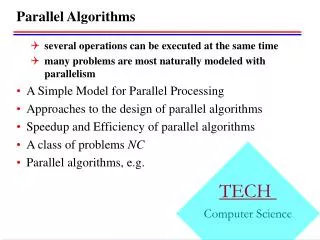
Introduction to parallel algorithms

1. Introduction to parallel algorithms COT 5410 – Spring 2004 Ashok Srinivasan www.cs.fsu.edu/~asriniva Florida State University

2. Outline • Background • Primitives • Algorithms • Important points

3. Background • Terminology • Time complexity • Speedup • Efficiency • Scalability • Communication cost model

4. Sequential Parallel - bad Parallel - ideal Parallel - realistic Time complexity • Parallel computation • A group of processors work together to solve a problem • Time required for the computation is the period from when the first processor starts working until when the last processor stops

5. Other terminology • Speedup: S = T1/TP • Efficiency: E = S/P • Work: W = P TP • Scalability • How does TP decrease as we increase P to solve the same problem? • How should the problem size increase with P, to keep E constant? • Notation • P = Number of processors • T1 = Time on one processor • TP = Time on P processors

6. Communication cost model • Processes spend some time doing useful work, and some time communicating • Model communication cost as • TC = ts + L tb • L = message size • Independent of location of processes • Any process can communicate with any other process • A process can simultaneously send and receive one message

7. I/O model • We will ignore I/O issues, for the most part • We will assume that input and output are distributed across the processors in a manner of our choosing • Example: Sorting • Input: x1, x2, ..., xn • Initially, xi is on processor i • Output xp1, xp2, ..., xpn • xpi on processor i • xpi< xpi+1

8. Primitives • Reduction • Broadcast • Gather/Scatter • All gather • Prefix

9. Reduction -- 1 x1 Compute x1 + x2 + ... + xn • Tn = n-1 + (n-1)(ts+tb) • Sn = 1/(1 + ts + tb) x2 xn x3 x4

10. Reduction -- 2 • Tn = n/2-1 + (n/2-1)(ts+ tb) + (ts+ tb) + 1 = n/2 + n/2 (ts+ tb) • Sn ~ 2/(1 + ts+ tb) x1 Reduction-1 for {x1, ... xn/2} xn/2+1 Reduction-1 for {xn/2+1, ... xn}

11. Reduction -- 3 xn/2+1 x1 • Apply reduction-2 recursively • * Divide and conquer • Tn ~ log2n + (ts+ tb) log2n • Sn ~ (n/ log2n) x 1/(1 + ts+ tb) • Note that any associative operator can be used in place of + Reduction-1 for {x1, ... xn/2} Reduction-1 for {xn/2+1, ... xn} xn/4+1 xn/2+1 x3n/4+1 x1 Reduction-1 for {x1, ... xn/4} Reduction-1 for {xn/4+1, ... xn/2} Reduction-1 for {xn/2+1, ... x3n/4} Reduction-1 for {x3n/4+1, ... xn}

12. Parallel addition features • If n >> P • * Each processor adds n/P distinct numbers • Perform parallel reduction on P numbers • TP ~ n/P + (1 + ts+ tb) log P • Optimal P obtained by differentiating wrt P • Popt ~ n/(1 + ts+ tb) • If communication cost is high, then fewer processors ought to be used • E = [1 + (1+ ts+ tb) P logP/n]-1 • * As problem size increases, efficiency increases • * As number of processors increases, efficiency decreases

13. A A A A, B, C, D A B A C A D Broadcast Gather A, B, C, D A A A, B, C, D B B A, B, C, D C C A, B, C, D D D A, B, C, D Scatter All Gather Some common collective operations

14. Broadcast • T ~ (ts+ Ltb) logP • L: Lenght of data x7 x8 x1 x1 x2 x3 x4 x1 x3 x2 x4 x5 x6 x1 x5 x3 x7 x2 x6 x4 x8 x1 x2

15. x18 x14 x58 x12 x34 x56 x78 x1 x2 x3 x4 x5 x6 x7 x8 Gather/Scatter Note: Si=0log P–1 2i = (2 log P – 1)/(2–1) = P-1 ~ P • Gather: Data move towards the root • Scatter: Review question • T ~ ts logP + PLtb 4L 2L 2L L L L L

16. All gather x7 x8 x3 x4 x5 x6 L x1 x2 • Equivalent to each processor broadcasting to all the processors

17. All gather x78 x78 x34 x34 2L x56 x56 L x12 x12

18. All gather x58 x58 x14 x14 2L x58 x58 L 4L x14 x14

19. All gather x18 x18 • Tn ~ ts logP + PLtb x18 x18 2L x18 x18 L 4L x18 x18

20. Review question: Pipelining • * Useful when repeatedly and regularly performing a large number of primitive operations • Optimal time for a broadcast = log P • But doing this n times takes n log P time • Pipelining the broadcasts takes n + P time • Almost constant amortized time per broadcast • if n >> P • n + P << n log P when n >> P • Review question: How can you accomplish this time complexity?

21. Sequential prefix • Input • Values xi , 1 < i < n • Output • Xi = x1 * x2 * ... * xi, 1 < i < n • * is an associative operator • Algorithm • X1 = x1 • for i = 2 to n • Xi = Xi-1 * xi

22. Parallel prefix • Define f(a,b) as follows • if a == b • Xi = xi, on ProcPi • Xi = xi, on Proc Pi • else • compute in parallel • f(a,(a+b)/2) • f((a+b)/2+1,b) • Pi and Pj send Xi and Xj to each other, respectively • a < i < (a+b)/2 • j = i + (a+b)/2 • Xi = Xi*Xj on Pi • Xj = Xi*Xj on Pj • Xj = Xi*Xj on Pj • Input • Processor i has xi • Output • Processor i has x1 * x2 * ... * xi • Divide and conquer • f(a,b) yields the following • Xi = xa *... * xi, Proc Pi • Xi = xa *... * xb, Proc Pi • a < i < b • f(1,n) solves the problem • T(n) = t(n/2) + 2 + (ts+tw) => T(n) = O(log n) • An iterative implementation improves the constant

23. Iterative parallel prefix example x0 x1 x2 x3 x4 x5 x6 x7 x01 x12 x23 x34 x45 x56 x67 x02 x03 x14 x25 x36 x47 x04 x05 x06 x07

24. Algorithms • Linear recurrence • Matrix vector multiplication

25. Linear recurrence • Determine each xi, 2 < i < n • xi = ai xi-1 + bi xi-2 • x0 = x0, x1 = x1 • Sequential solution • for i = 2 to n • xi = ai xi-1 + bi xi-2 • Follows directly from the recurrence • This approach is not easily parallelized

26. Linear recurrence in parallel • Given xi = ai xi-1 + bi xi-2 • x2i = a2i x2i-1 + b2i x2i-2 • x2i+1 = a2i+1 x2i + b2i+1 x2i-1 • Rewrite this in matrix form x2i x2i+1 x2i-2 x2i-1 b2i a2i a2i+1b2ib2i+1 + a2i+1 a2i Ai Xi-1 Xi • Xi = Ai Ai-1 ... A1X0 • This is a parallel prefix computation, since matrix multiplication is associative • Solved in O(log n) time

27. Matrix-vector multiplication • c = A b • Often performed repeatedly • bi = A bi-1 • We need same data distribution for c and b • One dimensional decomposition • Example: row-wise block striped for A • b and c replicated • Each process computes its components of c independently • Then all-gather the components of c

28. 1-D matrix-vector multiplication • Each process computes its components of c independently • Time = Q(n2/P) • Then all-gather the components of c • Time = ts log P + tb n • Note: P < n c: Replicated A: Row-wise b: Replicated

29. 2-D matrix-vector multiplication C0 A00 A01 A02 A03 B0 C1 A10 A11 A12 A13 B1 • Processes Pi0 sends Bi to P0i • Time: ts + tbn/P0.5 • Processes P0j broadcast Bj to all Pij • Time = ts log P0.5 + tb n log P0.5 / P0.5 • Processes Pij compute Cij = AijBj • Time = Q(n2/P) • Processes Pij reduce Cij on to Pi0, 0 < i < P0.5 • Time = ts log P0.5 + tb n log P0.5 / P0.5 • Total time = Q(n2/P + ts log P + tb n log P / P0.5 ) • P < n2 • * More scalable than 1-dimensional decomposition C2 A20 A21 A22 A23 B2 C3 A30 A31 A32 A33 B3

30. Important points • Efficiency • Increases with increase in problem size • Decreases with increase in number of processors • Aggregation of tasks to increase granularity • Reduces communication overhead • Data distribution • 2-dimensional may be more scalable than 1-dimensional • Has an effect on load balance too • General techniques • Divide and conquer • Pipelining