Squared coefficient of variation
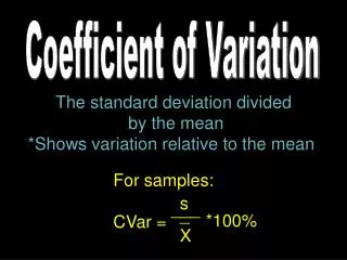
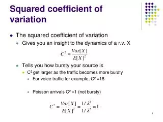
Squared coefficient of variation. The squared coefficient of variation Gives you an insight to the dynamics of a r.v. X Tells you how bursty your source is C 2 get larger as the traffic becomes more bursty For voice traffic for example, C 2 =18 Poisson arrivals C 2 =1 (not bursty).

Squared coefficient of variation
E N D
Presentation Transcript
Squared coefficient of variation • The squared coefficient of variation • Gives you an insight to the dynamics of a r.v. X • Tells you how bursty your source is • C2 get larger as the traffic becomes more bursty • For voice traffic for example, C2 =18 • Poisson arrivals C2 =1 (not bursty)
Erlang, Hyper-exponential, and Coxian distributions • Mixture of exponentials • Combines a different # of exponential distributions • Erlang • Hyper-exponential • Coxian μ μ μ E4 μ Service mechanism μ1 P1 μ2 H3 P2 P3 μ3 μ μ μ μ C4
Erlang distribution: analysis 1/2μ 1/2μ • Mean service time • E[Y] = E[X1] + E[X2] =1/2μ + 1/2μ = 1/μ • Variance • Var[Y] = Var[X1] + Var[X2] = 1/4μ2 v +1/4μ2 = 1/2μ2 E2
Squared coefficient of variation: analysis constant exponential C2 • X is a constant • X = d => E[X] = d, Var[X] = 0 => C2 =0 • X is an exponential r.v. • E[X]=1/μ; Var[X] = 1/μ2 => C2 = 1 • X has an Erlang r distribution • E[X] = 1/μ, Var[X] = 1/rμ2 => C2 = 1/r • fX*(s) = [rμ/(s+rμ)]r Erlang 0 1 Hypo-exponential
Probability density function of Erlang r • Let Y have an Erlang r distribution • r = 1 • Y is an exponential random variable • r is very large • The larger the r => the closer the C2 to 0 • Ertends to infintiy => Y behaves like a constant • E5 is a good enough approximation
Generalized Erlang Er • Classical Erlang r • E[Y] = r/μ • Var[Y] = r/μ2 • Generalized Erlang r • Phases don’t have same μ … rμ rμ rμ Y … μ1 μ2 μr Y
Generalized Erlang Er: analysis • If the Laplace transform of a r.v. Y • Has this particular structure • Y can be exactly represented by • An Erlang Er • Where the service rates of the r phase • Are minus the root of the polynomials
Hyper-exponential distribution μ1 P1 • P1 + P2 + P3 +…+ Pk =1 • Pdf of X? μ2 X P2 . . Pk μk
Hyper-exponential distribution:1st and 2nd moments • Example: H2
Hyper-exponential: squared coefficient of variation • C2 = Var[X]/E[X]2 • C2 is greater than 1 • Example: H2 , C2 > 1 ?
Coxian model: main idea • Idea • Instead of forcing the customer • to get r exponential distributions in an Er model • The customer will have the choice to get 1, 2, …, r services • Example • C2 : when customer completes the first phase • He will move on to 2nd phase with probability a • Or he will depart with probability b (where a+b=1) a b
Coxian model μ2 μ3 μ4 μ1 a2 a3 a1 b1 b2 b3 μ1 b1 a1 b2 μ1 μ2 a1 a2 b3 μ1 μ2 μ3 a1 a2 a3 μ1 μ2 μ3 μ4
Coxian distribution: Laplace transform • Laplace transform of Ck • Is a fraction of 2 polynomials • The denominator of order k and the other of order < k • Implication • A Laplace transform that has this structure • Can be represented by a Coxian distribution • Where the order k = # phases, • Roots of denominator = service rate at each phase
Coxian model: conclusion • Most Laplace transforms • Are rational functions • => Any distribution can be represented • Exactly or approximately • By a Coxian distribution
Coxian model: dimensionality problem • A Coxian model can grow too big • And may have as such a large # of phases • To cope with such a limitation • Any Laplace transform can be approximated by a Coxian 2 • The unknowns (a, μ1, μ2) can be obtained by • Calculating the first 3 moments based on Laplace transform • And then matching these against those of the C2 a μ1 μ2 b=1-a
Some Properties of Coxian distribution • Let X be a random variable • Following the Coxian distribution • With parameters µ1,µ2, and a • PDF of this distribution • Laplace transform
First three moments of Coxian distribution • By using • We have • Squared Coefficient of variation • => • For a Coxian k distribution =>
Approximating a general distribution • Case I: c2> 1 • Approximation by a Coxian 2 distribution • Method of moments • Maximum likelihood estimation • Minimum distance estimation • Case II: c2< 1 • Approximation by a generalized Erlang distribution
Method of moments • The first way of obtaining the 3 unknowns (μ1μ2 a) • 3 moments method • Let m1, m2, m3 be the first three moments • of the distribution which we want to approximate by a C2 • The first 3 moments of a C2 are given by • by equating m1=E(X), m2=E(X2), and m3 = E(X3), you get
3 moments method • The following expressions will be obtained • Let X=µ1+µ2and Y=µ1µ2, solving for X and Y • and • => and • However, • The following condition • has to hold: X2 – 4Y >= 0 • => • Otherwise, resort to a two moment approximation
Two-moment approximation • If the previous condition does not hold • You can use the following two-moment fit • General rule • Use the 3 moments method • If it doesn’t do => use the 2 moment fit approximation
Maximum likelihood estimation • A sample of observations • from arbitrary distribution is needed • Let sample of size N be x1, x2, …, xN • Likelihood of sample is: • Where is the pdf of fitted Coxian distribution • Product to summation transformation • Maximum likelihood estimate: • Maximize L subject to • and
Minimum distance estimation • Objective • Minimize distance • Between fitted distribution and observed one • => a sample observation of size N x1, x2, …, xN • is needed • Computing formula for the distance • , where • X(i) is the ith order statistic and Fθ(x) is the fitted C2 • A solution is obtained by minimizing the distance • No closed form solution exists • => a non-linear optimization algorithm can be used
Concluding remarkson case I • If exact moments • of arbitrary distribution are known • Then the method of moments should be used • Otherwise, • Maximum likelihood or minimum distance estimations • Give better results
Case II: c2 < 1 • Generalized Erlang k can be used • To approximate the arbitrary distribution • In this case • Service ends with probability 1-a or • Continues through remaining k-1 phases with probability a • The number of stages k should be such that • Once k is fixed, parameters can be obtained as: