Historical Perspective on Network Interconnection: From Early Machines to Modern Algorithms
Explore the evolution of network interconnection from early machines to contemporary algorithms. This overview discusses the significance of bi-directional communication, the “store and forward” method, and the importance of network topology in minimizing latency and hops. Delve into how networks can be likened to streets, where links are streets, switches are intersections, and routing algorithms function as travel plans. The text also highlights performance metrics such as latency and bandwidth and examines different network topologies, including linear arrays, meshes, tori, and hypercubes, establishing their relevance in optimization.

Historical Perspective on Network Interconnection: From Early Machines to Modern Algorithms
E N D
Presentation Transcript
Historical Perspective • Early machines were: • Collection of microprocessors. • Communication was performed using bi-directional queues between nearest neighbors. • Messages were forwarded by processors on path. • “Store and forward” networking • There was a strong emphasis on topology in algorithms, in order to minimize the number of hops = minimize time
Network Analogy • To have a large number of transfers occurring at once, you need a large number of distinct wires. • Networks are like streets: • Link = street. • Switch = intersection. • Distances (hops) = number of blocks traveled. • Routing algorithm = travel plan. • Properties: • Latency: how long to get between nodes in the network. • Bandwidth: how much data can be moved per unit time. • Bandwidth is limited by the number of wires and the rate at which each wire can accept data.
Design Characteristics of a Network • Topology (how things are connected): • Crossbar, ring, 2-D and 3-D meshs or torus, hypercube, tree, butterfly, perfect shuffle .... • Routing algorithm (path used): • Example in 2D torus: all east-west then all north-south (avoids deadlock). • Switching strategy: • Circuit switching: full path reserved for entire message, like the telephone. • Packet switching: message broken into separately-routed packets, like the post office. • Flow control (what if there is congestion): • Stall, store data temporarily in buffers, re-route data to other nodes, tell source node to temporarily halt, discard, etc.
Performance Properties of a Network: Latency • Diameter: the maximum (over all pairs of nodes) of the shortest path between a given pair of nodes. • Latency: delay between send and receive times • Latency tends to vary widely across architectures • Vendors often report hardware latencies (wire time) • Application programmers care about software latencies (user program to user program) • Observations: • Hardware/software latencies often differ by 1-2 orders of magnitude • Maximum hardware latency varies with diameter, but the variation in software latency is usually negligible • Latency is important for programs with many small messages
Routing and control header Data payload Error code Trailer Performance Properties of a Network: Bandwidth • The bandwidth of a link = w * 1/t • w is the number of wires • t is the time per bit • Bandwidth typically in Gigabytes (GB), i.e., 8* 220 bits • Effective bandwidth is usually lower than physical link bandwidth due to packet overhead. • Bandwidth is important for applications with mostly large messages
Performance Properties of a Network: Bisection Bandwidth • Bisection bandwidth: bandwidth across smallest cut that divides network into two equal halves • Bandwidth across “narrowest” part of the network not a bisection cut bisection cut bisection bw= link bw bisection bw = sqrt(n) * link bw • Bisection bandwidth is important for algorithms in which all processors need to communicate with all others
Network Topology • In the past, there was considerable research in network topology and in mapping algorithms to topology. • Key cost to be minimized: number of “hops” between nodes (e.g. “store and forward”) • Modern networks hide hop cost (i.e., “wormhole routing”), so topology is no longer a major factor in algorithm performance. • Example: On IBM SP system, hardware latency varies from 0.5 usec to 1.5 usec, but user-level message passing latency is roughly 36 usec. • Need some background in network topology • Algorithms may have a communication topology • Topology affects bisection bandwidth.
Linear and Ring Topologies • Linear array • Diameter = n-1; average distance ~n/3. • Bisection bandwidth = 1 (in units of link bandwidth). • Torus or Ring • Diameter = n/2; average distance ~ n/4. • Bisection bandwidth = 2. • Natural for algorithms that work with 1D arrays.
Meshes and Tori Two dimensional mesh • Diameter = 2 * (sqrt(n ) – 1) • Bisection bandwidth = sqrt(n) Two dimensional torus • Diameter = sqrt(n ) • Bisection bandwidth = 2* sqrt(n) • Generalizes to higher dimensions (Cray T3D used 3D Torus). • Natural for algorithms that work with 2D and/or 3D arrays.
Hypercubes • Number of nodes n = 2d for dimension d. • Diameter = d. • Bisection bandwidth = n/2. • 0d 1d 2d 3d 4d • Popular in early machines (Intel iPSC, NCUBE). • Lots of clever algorithms. • Greycode addressing: • Each node connected to d others with 1 bit different. 110 111 010 011 100 101 000 001
Trees • Diameter = log n. • Bisection bandwidth = 1. • Easy layout as planar graph. • Many tree algorithms (e.g., summation). • Fat trees avoid bisection bandwidth problem: • More (or wider) links near top. • Example: Thinking Machines CM-5.
O 1 O 1 O 1 O 1 Butterflies with n = (k+1)2^k nodes • Diameter = 2k. • Bisection bandwidth = 2^k. • Cost: lots of wires. • Used in BBN Butterfly. • Natural for FFT. butterfly switch multistage butterfly network
Topologies in Real Machines older newer Many of these are approximations: E.g., the X1 is really a “quad bristled hypercube” and some of the fat trees are not as fat as they should be at the top
Latency and Bandwidth Model • Time to send message of length n is roughly • Topology is assumed irrelevant. • Often called “a-b model” and written • Usually a >> b >> time per flop. • One long message is cheaper than many short ones. • Can do hundreds or thousands of flops for cost of one message. • Lesson: Need large computation-to-communication ratio to be efficient. Time = latency + n*cost_per_word = latency + n/bandwidth Time = a + n*b a + n*b << n*(a + 1*b)
Alpha-Beta Parameters on Current Machines • These numbers were obtained empirically a is latency in usecs b is BW in usecs per Byte How well does the model Time = a + n*b predict actual performance?
End to End Latency Over Time • Latency has not improved significantly, unlike Moore’s Law • T3E (shmem) was lowest point – in 1997 Data from Kathy Yelick, UCB and NERSC
Send Overhead Over Time • Overhead has not improved significantly; T3D was best • Lack of integration; lack of attention in software Data from Kathy Yelick, UCB and NERSC
Bandwidth Chart Data from Mike Welcome, NERSC
Results: EEL and Overhead Data from Mike Welcome, NERSC