CHP-7 GRAPH
CHP-7 GRAPH. INTRODUCTION. A graph is a special types of another important non-linear data structure called graph. It differ from tree in the sense that it represents the relationship that is not necessary hierarchical in nature, that is node may have more than one parent.

CHP-7 GRAPH
E N D
Presentation Transcript
INTRODUCTION • A graph is a special types of another important non-linear data structure called graph. • It differ from tree in the sense that it represents the relationship that is not necessary hierarchical in nature, that is node may have more than one parent.
1.DEFINITION & TERMINOLOGY • A graph denoted by G(V,E) consists of a pair of two non-empty sets V and E, where V is a set of vertices (nodes) and E is a set of edges. • In below fig. the set of vertices is {1,2,3,4,5,6} and set of edges is{(1,2),(2,3),(1,3),(2,5),(3,5),(4,5),(3,4),(4,6)} 2 5 1 6 3 4 Fig.7.1(a) Undirected Graph
This Graph is undirected graph since there is no direction associated with its edges. • In Undirected Graph ,the pair of vertices (1,2) and (2,1) represent same edge( means both are same). • See fig.
If direction is associated with each edge ,the graph is known as directed graph(digraph). • For example fig.7.1(b) shows a directed graph in which directions are indicated using arrows. • Here, the pair of vertices(1,2) and (2,1) represents the different edge(means both are different). 1 4 2 3 Fig.7.1(b) Directed Graph
TERMINOLOGIES • ADJACENT VERTICES: two vertices x and y are said to be adjacent ,if there is an edge from x to y or from y to x. In fig.7.1(a) vertices 1 and 3, 2 and 5 are adjacent,but 1 and 5 are not. • DEGREE: the degree of a vertex x, denoted as degree(x), is the number of edges containing x. In fig.7.1(a) the degree of vertex 2 is 3. • Degree(x) can be zero also which represents that vertex x does not belong to any edge. • In this case ,vertex is called isolated vertex. In below fig. 4 is isolated vertex. 2 1 4 3
TERMINOLOGIES • PATH: a path of length k from vertex x to y is defined as a sequence of k+1 vertices v1,v2,……,vk+1 such that v1=x ,vk+1=y and vi is adjacent to vi+1 for i=1,2,……,k+1. • For example in fig.7.1(a) there is a path of length 2 from vertex 1 to 5 and path of 4 from vertex 1 to 6. • If v1=vk+1 then path is said to be closed. • If all vertices are distinct except v1 and vk+1,which may be same, then path is said to be simple.
TERMINOLOGIES • CYCLE:A cycle is a closed simple path. if a graph contains a cycle, it is called cyclic graph otherwise. acyclic graph. • LOOP: An edge is a loop if its starting and ending vertex are same. For example,In Figure 7. 1 (c) edge (4.4) is a loop. 2 6 1 4 3 5 7.1(c)Disconnected Graph
TERMINOLOGIES • Connected graph: A graph is said to be connected if there is a path between any two of its vertices, that is. there is no isolated vertex. For example, the graph shown in Figure 7. l( a ) is connected whereas the graph shown in Figure 7.1(c) is not connected. • Weighted graph: A graph is said to be weighted If a non-negative number (called weight) is associated with each edge. This weight may represent distance between two vertices or cost of moving along that edge.. Figure 7.1(d) illustrates a weighted graph. Fig.7.1(d) Weighted Graph 6 5 5 2 1 9 8 4 3 4 3
TERMINOLOGIES(FOR DIRECT GRAPH ONLY) • Indegree of a vertex: Indegree of a vertex x, denoted by indeq (x) refers to the number of edges terminating at x. For examp1e. in directed graph shown in Figure 7. 1(b),indeg(2) = 1. • Outdegree of a vertex: Outdegree of a vertex x, denoted by outdeq (x) refers to the number of edges originating at x. For examp1e. in directed graph shown in Figure 7. 1(b),outdeg(2) = 2. • A directed graph is said to be strongly connected if for every pair of vertices <x,y>,there exits a directed path from x to y and from y to x (see fig.7.1(e) ). • A directed graph is said to be weakly connected if for every pair of vertices <x,y>,there exits a path from either x to y or from y to x.(see fig.7.1(f)). Fig.7.1(f) Fig.7.1(e) 2 3 2 3 5 5 1 1 4 4
2.REPRESENTATIONS OF GRAPH • Two types of representations can be used to maintain a graph in memory which are sequential (array) and linked representation. • In sequential representation ,a graph is represented by means of adjacency matrix while in linked representation ,it is represented by means of adjacency lists.
Adjacency Matrix Representation • Given a Graph G (V, E) with n Vertices, the adjacency matrix A for this graph is a n x n matrix such that Aij= 1,if there is edge from vi to vj where ,1<=i<=n 0,if there is no edge 1<=j<=n • This matrix is also known as bit matrix or boolean matrix since it contains only two values 0 and 1. • The adjacency matrices for the graphs 7. 1(a) and 7.1 (b) are shown in fig. 7.2.
Adjacency Matrix Representation • Observe that the adjacency matrix for an undirected graph is symmetric,that is the upper and tower triangles of matrix are same. • However, it does not hold always true for the directed graph. • Note that in the adjacency matrix of directed graph, the total number of I 's tells the number Of edges and the number of 1’s in row tells the out degree of corresponding vertex. • Although adjacency matrix is a simple way to represent a graph but it needs n2 bits to represent a graph with n vertices. • in case Of undirected graph, by storing only upper or lower triangle of the matrix, this space can be reduced to half. • However, directed graph is not Symmetric always. so it takes n2 space for most of the graph problems.
Adjacency Lists • In adjacency list representation ,the graph is stored as a linked structure. • In this representation ,for each vertex, a linked list (known as adjacency list) is maintained that stores its adjacent vertices. • That is ,for n vertices in a graph, there will be n adjacency lists. • Each list has a header node that points to its corresponding adjacency list. • The header nodes are stored sequentially to provide easy access to adjacency list for each vertex. • The adjacency lists for graphs 7.1(a) and 7.1(b) are shown in fig. 7.3(a) and 7.3(b) respectively.
3.ELEMENTARY GRAPH OPERATIONS • Following are basic operations that can be performed on graph: (1)Create operation: to create an empty graph. (2)Input operation: to enter graph information. (3)Display operation: to display graph information. (4)Delete operation: to delete a graph. To store the information of graph ,the node is defined using structure named nodes as follows. Struct node { int info; struct node *next; }Node;
4 TRAVERSING A GRAPH • One of the common operations that can be performed on graphs is traversing, that is, visiting all vertices that are reachable from a given vertex. • The most commonly used methods for traversing a graph are depth-first search and breadth-first search.
Depth-First Search(DFS) • In depth-first search, starting from any vertex, a single path P of the graph is traversed until a vertex is found whose all-adjacent vertices have already been visited. • The search then backtracks on the path P until a vertex with unvisited adjacent vertices is found and then begins traversing a new path p' starting from that vertex and so on. • This process continues until all the vertices of graph are visited. • Note that there is always a possibility that a vertex can be traversed more than one time. • Thus, it is required to keep track whether the vertex is already visited.
Depth-First Search(DFS)(Cont.) • For example, the depth-first search for the graph shown in Figure 7.4(a) results in sequence of vertices 1,2,4,3,5,6 which is obtained as follows: 1.Visit a vertex, say, 1. 2. Its adjacent vertices are 2,3,4 and 6. Select any unvisited vertex, say, 2. 3. Its adjacent vertices are 1 and 4. Since vertex 1 is already visited, select unvisited vertex 4. 4. Its adjacent vertices are 1, 2 and 3. Since vertices 1 and 2 are already visited, select unvisited vertex 3. 5. Its adjacent vertices are 1,4,5 and 6. Since vertices 1 and 4 are already visited, select an unvisited vertex, say, 5. 6. Its adjacent vertices are 3 and 6. Select the unvisited vertex 6. Since all the adjacent vertices of vertex 6 are already visited, backtrack to visited adjacent vertices to find if there is any unvisited vertex. Since, all the vertices are visited, algorithm terminates
Depth-First Search(DFS)(Cont.) • To implement depth-first search, an array of pointers arr _ptr to store the address of the first vertex in each adjacency list and a boolean-valued array visi ted to keep track of the visited vertices are maintained. • Initially, all the values of visited array are initialized to Fa1s e to indicate that no vertex has been visited yet. • As soon as a vertex is visited,its value is changed to True in array visi ted. Following is the recursive algorithm for depth-first search.
Breadth-First-Search(BFS) • In breadth-first search, starting from any vertex, all its adjacent vertices are traversed. • Then anyone of adjacent vertices is selected and all its adjacent vertices that have not been visited yet are traversed. • This process continues until all the vertices have been visited. • For example, the breadth-first search for the graph shown in Figure 7.4(a) results in sequence 1,2,3,4,.6,5 which is obtained as follows:
Breadth-First-Search(BFS)(Cont.) 1.Visit a vertex, say, 1. 2. Its adjacent vertices are 2, 3,4 and 6. Visit all these vertices one by one. select any vertex, say, 2 and find its adjacent vertices. 3. Since all the adjacent vertices for 2, that is, 1 and 4 are already visited, select vertex 3. 4. Its adjacent vertices are 1, 5 and 6. Visit 5 as 1 and 6 are already visited. 5. Since all the vertices are visited, the process is terminiated.
Breadth-First-Search(BFS)(Cont.) • The implementation of breadth-first search is quite similar to the implementation of depth-first search. • The difference is that former uses a queue instead of stack (either implicitly via recursion or explicitly) to store the vertices of each level as they are visited. • These vertices are then taken one by one and their adjacent vertices are visited and so on until all the vertices have been visited. The algorithm terminates when the queue becomes empty.
5.APPLICATIONS OF GRAPHS • The graphs have found application in diverse areas. Various real-life situations like traffic flow, analysis of electrical circuits, finding shortest routes, applications related with computation,etc., can be easily managed by the graphs. • Some of the applications of graphs like topological sorting, minimum spanning trees and finding shortest path are discussed here.
Topological Sorting • The topological sort of a directed acyclic graph is a linear ordering of the vertices such that if there exists a path from vertex x to y, then x appears before y in the topological sort. • Formally, for a directed acyclic graph G = (V, E), where V = {Vl, V2, V3, . . , Vn }, if there exists a path from any Vi to Vj then Vi appears before Vj in the topological sort. • An acyclic directed graph can have more than one topological sort. • For example, two different topological sorts for the graph illustrated in Figure 7.5 are (1, 4,2, 3) and (1, 2, 4, 3).
Topological Sorting(Cont.) • Clearly, if a directed graph contains a cycle, topological ordering of vertices is not possible. • It is because for any two vertices Vi and Vj in the cycle, Vi precedes Vj as well as Vj precedes Vi. • To exemplify this, consider a simple cyclic directed graph shown in Figure 7.6. • The topological sort for this graph is (1, 2, 3, 4) (assuming the vertex 1 as starting vertex). • Now, since there exists a path from the vertex 4 to 1, then according to the definition of topological sort, the vertex 4 must appear before the vertex 1, which contradicts the topological sort generated for this graph. • Hence, topological sort can exist only for the acyclic graph.
Topological Sorting(Cont.) • In an algorithm to find the topological sort of an acyclic directed graph, the indegree of the vertices is considered. • Following are the steps that are repeated until the graph is empty. 1. Select any vertex Vi with 0 indegree. 2. Add vertex Vi to the topological sort (initially the topological sort is empty). 3. Remove the vertex Vi along with its edges from the graph and decrease the indegree of each adjacent vertex of Vi by one. • To illustrate this algorithm, consider an acyclic directed graph shown in Figure 7.7.
Minimum Spanning Trees • A spanning tree of a connected graph G is a tree that covers all the vertices and the edges required to connect those vertices in the graph. • Formally, a tree T is called a spanning tree of a conneected graph G if the following two conditions hold. 1. T contains all the vertices of G and 2. all the edges of T are subsets of edges of G. • For a given graph G with n vertices, there can be many spanning trees and each tree will have n-l edges. For example, consider a graph as shown in Figure 7.10. • Since this graph has 4 vertices, each spanning tree must have 4-1 = 3 edges. Some of the spanning trees for this graph are shown in Figure 7.11. • Observe that in spanning trees, there exists only one path between any two vertices and insertion of any other edge in the spanning tree results in a cycle.
Minimum Spanning Trees(Cont.) • For a connected weighted graph G, it is required to construct a spanning tree T such that the sum of weights of the edges in T must be minimum. Such a tree is called a minimum spanning tree. • There are various approaches for constructing a minimum spanning tree. • One such approach has been given by Kruskal. In this approach, initially, all the vertices n of the graph are considered as distinct partial tree having one vertex. • The minimum spanning tree is constructed by repeatedly inserting one edge at a time until exactly n -1 edges are inserted. • The edges are inserted in the increasing order of their costs. Further, an edge is inserted in the tree only if its inclusion does not form a cycle. • Consider an undirected weighted connected graph shown in Figure 7.12. • In order to construct the minimum spanning tree T for this graph, the edges must be included in the • order (1,3), (1, 2), (1, 6), (4, 6), (3, 6), (2, 6), (3, 4), (1, 5), (3, 5) and (4,5). • This sequence of edges corresponds to the increasing order of weights (3, 4, 5, 6, 7, 8, 9, 12, 14 and 15). • The first four edges (1, 3), (1, 2), (1, 6) and (4,6) are included in T. • The next edge that is to be inserted in order of cost is (3, 6). Since, its inclusion in the 'tree forms a cycle, it is rejected. For same reason, the edges (2, 6) and (3, 4) are rejected. • Finally, on the insertion of the edge (1,5), T has n-l edges. • Thus, the algorithm terminates and the generated tree is a minimum spanning tree. • The weight of this minimum spanning tree is 30. All the steps are shown in Figure 7.13.
Shortest Path • There are various algorithms to find the shortest path between any two vertices of a graph. • One such algorithm was proposed by E.W. Dijkstra. • According to this algorithm, initially, the adjacency matrix showing the cost of edges of the graph is constructed. • Starting from any vertex (say, V), the path of other vertices from Vi is calculated. • Then the cost of each path is compared; if the cost of a path is smaller than that of previous cost, it is replaced with the new cost. This process is continued until all the vertices of graph are taken into account. • To understand the working of Dijkstra's algorithm, consider a directed weighted graph having 4 vertices shown in Figure 7.14.
Shortest Path(Cont.) • For this graph, the adjacency matrix (where, the '-' indicates that there is no direct path between the vertices) and the matrix representing the path between the vertices (where, the '-' indicates that till now path is not determined) are as follows. • Starting from the vertex 1, calculate the cost of all the paths that can be visited via vertex • From the graph, it is clear that the paths that can be visited via vertex 1 are 2-1-3, 3-1-3,2-1-4 and 3-1-4. Among these paths, the cost of the path between vertices 2 and 4 is less as compared to the previous one, so it must be replaced in the adjacency matrix. Also, a path between vertices 3 and 3 is found which must be added in the adjacency matrix. The adjacency matrix after considering vertex 1 is as follows. Here, the values that are underlined and bold indicate that they are either added or replaced.
Shortest Path(Cont.) • Now, consider the vertex 2. The resultant adjacency matrix and the matrix representing the path are as follows. After considering vertex 2, neither any new path nor a path whose cost is less than the current ones is found. Thus, the adjacency matrix remains the same. • Similarly, the adjacency matrix and the matrix representing the path after considering vertex 3 are as follows. • Finally, the adjacency matrix and the matrix representing the path after considering vertex 4 are as follows. Here, the adjacency matrix and the matrix representing path show the cost of the shortest path and the shortest path, respectively, between any two vertices. Note that the' -' indicates that vertex 2 is unreachable.