
Understanding the Definite Integral and Riemann Sums: Continuity and Applications
This chapter delves into the concept of the definite integral, focusing on continuous functions defined over the interval [a, b]. It explains the Riemann sum approach for approximating the integral, utilizing equal-width subintervals and sample points. Examples are provided, including calculations involving right endpoints, left endpoints, and midpoints with ( f(x) = x^2 ) over the interval [0, 1]. The chapter also outlines properties of integrals, including the linearity of integration and the evaluation of definite integrals through various methods.

Understanding the Definite Integral and Riemann Sums: Continuity and Applications
E N D
Presentation Transcript
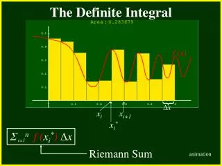
The Definite Integral CHAPTER 2 2.4 Continuity f (x) x xi xi+1 xi* i=1nf (xi*) x Riemann Sum animation
Definition of a Definite Integral If f is a continuous function defined for b x a we divide the interval [a,b] into subintervals of equal widthx =(b–a)/n. We let x0(= a), x1, x2 … xn ( = b) be the endpoints of these subintervals and we choose sample points x1*,x2*… xn*, so xi*lies in the ith subinterval [xi-1, xi]. Then the definite integralof f from a to b is b abf (x) dx = lim n0 i=1nf (xi*) x .
Example If f (x)= x2, 0 <= x <= 1, evaluate the Riemann sum with n = 4, taking the sample points to be right endpoints. Right endpoints animation
Example If f (x)= x2, 0 <= x <= 1, evaluate the Riemann sum with n = 4, taking the sample points to be left endpoints. Left endpoints animation
Example If f (x)= x2, 0 <= x <= 1, evaluate the Riemann sum with n = 4, taking the sample points to be midpoints. Midpoints animation
Midpoint Rule ba f (x) dx ni = 1 f (xi*) x = x [ f (x1) + … + f (xn)] where x = (b – a) / n and xi = ½ (xi-1 + xi) = midpoint of [xi-1, xi]. _ _ _
Properties of the Integral • abc dx = c(b – a), where c is any constant. • ab[ f (x) + g(x)]dx= abf (x) dx + abg(x) dx • 3. abc f (x) dx = c abf (x) dx , • 4. ab[ f (x) - g(x)]dx= abf (x) dx - abg(x) dx. • 6.abf (x) dx +abf (x) dx = abf(x) dx.


