Download
1 / 31
310 likes | 974 Vues
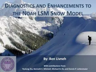
Diagnostics and Enhancements to the Noah LSM Snow Model . By: Ben Livneh With contributions from: Youlong Xia, Kenneth E. Mitchell, Michael B. Ek, and Dennis P. Lettenmaier. Presentation Overview. Motivation for the project. Model background Problem description Nature of model extensions

E N D
Diagnostics and Enhancements to the Noah LSM Snow Model By: Ben Livneh With contributions from: Youlong Xia, Kenneth E. Mitchell, Michael B. Ek, and Dennis P. Lettenmaier
Presentation Overview • Motivation for the project. • Model background • Problem description • Nature of model extensions • Off-line testing and results • Conclusions
Seasonal Reservoir Man-made Reservoir Motivation ≈ • Snow acts as a natural reservoir/buffer, to redistribute winter precipitation later into spring and summer when it is needed, important for water-supply, wildlife, etc… • Snow cover has a significant impact on numerical weather prediction; higher reflectance, altered surface thermal regime. Source www.waterencyclopedia.com Source www.wunderground.com Source www.usgcrp.com
Background – NOAH LSM • NOAH LSM: (NCEP, OSU, Air Force, Hydrologic research lab) • Land scheme for suite of weather and atmospheric models (NOAA), most versions of WRF. • Partitioning of radiation (H, LE) • Characterizes soil moisture, snow cover, etc… • Focus: snow cover very important to both land and atmosphere.
Problem • Negative in modeled snow water equivalent (SWE) bias noted in Noah LSM. • Important for coupled modeling (partitioning radiative inputs, fluxes) as well as hydrology (soil moisture anomalies and streamflow timing). Prompted offline testing of various model components Noah SWE (mm) Observed SWE (mm) Mitchell et al, 2004
Snow model structure (‘Control’: Noah v.2.7.1) • Single-layer snow model. • Linearized energy balance computation (computes skin temperature). • No liquid water retention • Uses a satellite-based spatially varying maximum snow albedo αMAX-satellite(Robinson and Kukla, 1985), constant value. • Turbulent exchange embodied in a surface exchange coefficient: CH • Partial snow coverage: Areal Depletion Snow cover frac. T1, WMAXαMAX, ρ, CH SWE/WMAX • Snowpack Energy Balance = Qn + Qh + Qe + Qg + Qa
Model Extensions 1. Evaluation of a snow albedo decay scheme that captures the varying characteristics of the snowpack, currently not addressed in the control model; 2. Implementation of an algorithm that accounts for liquid water storage and refreeze within the pore space of the snowpack; a process that is not represented in the control. • In addition, we report more limited sensitivity on: • Sensitivity of fractional snow coverage thresholds as they interact with albedo; • An alternative stability correction to the turbulent exchange physics.
Snow Albedo • CONTROL model considers a fixed maximum snow albedo value, based on the conversion of scene brightness (satellite imagery). • Does not account for seasonal variability, changes to the snow surface, etc.. DMSP Satellite image, 1979 Control Noah αMAX-satelliteconverted from DMSP satellite imagery (1979) Defense Meteorological Satellite Program (DMSP)
Snow Albedo Decay Scheme Snow albedo decay phenomenon confirmed by numerous studies (e.g Warren et al., 1980). Rate is determined by character of snow surface (metamorphism, recrystalization, debris, etc…). One method to quantify decay, via age of snow surface (equation). Seasonal decay rate (lower left) is faster during melt season: Shift between seasonal curves determined by snow surface temperature. Accumulation Season Melt Season Equation: αMAX ≈ 0.85; t: days since last snowfall; A,B: constants. Albedo decay scheme; based on Corps of Engineers, 1956; CA 10 Warren, S. G. and W. J. Wiscombe, 1980: A model for the spectral albedo of snow, II, Snow containing atmosphenc aerosols, J. Atmos. Sci., 37, 2734-2745. U.S. Army Corps Of Engineers, 1956: Summary report of the snow investigations, "Snow Hydrology", U. S. Army Engineer Division, North Pacific, 210 Custom House, Portland, Oregon 97209.
Snow Albedo – Additional Considerations • NCEP desire to preserve spatial variability of satellite αMAX value for decay scheme. • Hence an average value was used (midpoint between αMAX-satelliteand 0.85: weighting factor C = 0.5) • Required constraining lower bound of albedo (α≥ 40%) A: Accumulation season curve (αMAX = 0.85) B: Melt season curve (αMAX = 0.85) C: Accumulation season curve (C = 0.5) D: Melt season curve (C = 0.5) E: αMAX-satellite = constant (e.g. 52%) Lowerbound
Liquid Water Refreeze *Key difference in new energy balance • Important physical aspect (prevents snowmelt from going directly to runoff). • Requires extending the snowpack energy balance, utilizing a melt energy (cold content) approach: • Qm = Qn + Qh + Qe + Qg + Qa- ΔCC [W/m2] Where: Qm = Energy available for melt; Qn = Net radiation flux Qh = Sensible heat flux Qe = Latent heat flux Qg = Ground flux Qa = Advected heat flux ΔCC = Change in internal energy of the snow pack (cold content) → *New Term: Allows for monitoring of thermal inertia between successive time steps; necessary for controlling melt and refreeze processes; involves new variable: Tpack
Liquid Water Storage • Irreducible saturation, Swi, the maximum amount of liquid water a snowpack can hold, beyond which it will transmit water. • Tested several quantities (3.5 % SWE, 3 % total snowdepth, 4% of snowpack p.v.) • 4% of snow p.v. selected. Where: SWE = snow water equivalent; dsnow = snow depth, φ = porosity, ρ = density * Based on observations, Denoth et al., 2003
Additional Sensitivities • Wmax thresholds in control model: 0.04 m, 0.02 m (forest, non-forest) • In a *recent paper (based on comparison with albedo measurements) proposes: 0.20 m, 0.01 m (forest, non-forest) • This work combined with the great disparity in satellite based albedo formed the basis for sensitivity testing. * Wang Z, Zeng X (2009) Evaluation of snow albedo in land models for weather and climate studies. Journal of Applied Meteorology and Climatology: In Press Adjust areal depletion threshold for SWE; forest vs. non-forest. *Related to recent collaborative work at the University of Arizona.
Additional Sensitivities • Stability correction for turbulent exchange scheme to prevent excessive sublimation from occurring during stable conditions. • Extension of Slater et al. (2007) correction to momentum transfer (when RiB> 0) CH= CH*(1-RiB/2) CM= CM*(1-RiB/2) RiB: dimensionless form of bulk richardson number CH,CM: exchange coefficients for heat and momentum transfer, respectively.
Model evaluation strategy • Model performance evaluated through comparisons of off-line model simulations with observations. • 3 SNOTEL sites were chosen (western U.S.) to provide a reasonable cross section of snow types (continental, maritime, and intermediate) to represent regions where snow melt provides significant streamflow contributions (hydrology) • Large-scale model performance was evaluated using spatial plots of cumulative snow covered days (SCE) as compared to satellite data over CONUS domain at 1/8⁰. Duration of snow cover plays a vital role in partitioning atmospheric inputs (coupled model applications)
Albedo Decay αMAX-satellite • Improvements in SWE peak timing and magnitude at SNOTEL sites • Large-scale performance not consistent; generally improved at higher-elevation sites, however, highly correlated with satellite-based max snow albedo value (shown on next slide) αMAX = 0.85 αMAX → C=0.5 Comparison between albedo decay scheme (C=0.5) and control model
Albedo Decay (a) • Correlation between (a) albedo decay model performance vs. ‘control’, (b) αMAX-satellite , and (c) vegetation type. • For areas of high αMAX-satellite: albedo decay (C=0.5) case often falls below αMAX-satellite, yielding fewer snow covered days. • Relationship between areal depletion, αMAX and vegetation discussed later. (b) (c) Depiction of Noah forest vegetation classes
Melt Refreeze W.C. = 4% p.v. • Improved quantity and duration of SWE at SNOTEL sites. • Large-scale improvements nearly ubiquitous, however control out-performs the melt-refreeze version for some low albedo cases. • Altered energy balance and melt decision structure produce a slightly higher skin temperature in these cases, which can yield fewer snow covered days. W.C. = 3.5% SWE Comparison between melt/refreeze model and control model
Fractional Snow Coverage • Objective: test alternate Wmax values which accentuate the difference between forest and grasslands (including albedo-decay) to obtain a reasonable match with satellite values. • This was done by computing an average snow covered albedo for each grid-cell over the study period and comparing them with the CONTROL satellite-based snow albedo
Fractional Snow Coverage • Time-integrated plots less continuous than satellite value. • Wang and Zeng (2009) Wmax values together with albedo decay (C=0.5) yield a reasonable match.
Turbulent Exchange – Stability Correction • Reduction in sublimation over portions of the domain. However, high elevation sites (SNOTEL) results are inconclusive. • Further refinements appear to be in order. • Stability correction was considered as part of the ‘control’. Comparison between stability corrected model and uncorrected model
Optimal Model Performance • Inclusion of albedo decay (C=0.5), liquid water refreeze (W.C. = 4% p.v.) and adjusted Wmaxvalues. • Additionally, provide for separate albedos during partial snow coverage Comparison between suggested model extensions and control model
Conclusions • Negative SWE bias was addressed to improve model processes, evaluated at point-scale and large-scale. • Point scale testing revealed that albedo decay and melt-refreeze processes improve the quantity and timing of SWE (serve to improve streamflow predictions in snowmelt dominated basins) • Large-scale evaluation generally showed improvements in duration of snow cover; adjustment of areal depletion thresholds also provided for reasonable snow covered albedo estimates over the CONUS domain.
Acknowledgements Youlong Xia, Kenneth E. Mitchell, Michael B. Ek (NCEP) John Schaake (NWS) Ming Pan (Princeton) CPPA funding
Thank You Livneh, B., Y. Xia, K.E. Mitchell, M.B. Ek, and D.P. Lettenmaier, 2010: Noah LSM Snow Model Diagnostics and Enhancements, J. of Hydrometeorology, in press
New Snowpack Energy Balance Solution Procedure Qm = Qn + Qh + Qe + Qg + Qa- ΔCC • Procedure: • Guess *snowpack temperature (e.g. 273.15⁰K) for current time step and compute fluxes based on this temperature; • If residual Qm > 0 (energy surplus): melt an equivalent depth of water. First fill liquid water capacity within the pack; if melt water exceeds storage capacity, send to runoff. • If residual Qm < 0 (energy defecit): refreeze pack water, then cool pack with remaining energy deficit, if any. * Snowpack temperature is a new variable