Download
1 / 1
10 likes | 165 Vues
Noah LSM snow model diagnostics and enhancements. Ben Livneh 1 , Youlong Xia 2 , Michael Ek 2 , Ken Mitchell 2 , and Dennis Lettenmaier 1

E N D
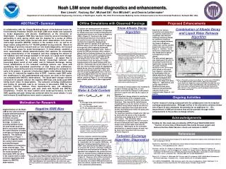
Noah LSM snow model diagnostics and enhancements. Ben Livneh1, Youlong Xia2, Michael Ek2, Ken Mitchell2,and Dennis Lettenmaier1 1Department of Civil and Environmental Engineering, University of Washington, Seattle, WA, USA 2Environmental Modeling Center, National Centers for Environmental Prediction, Suitland, MD, USA. ABSTRACT - Summary Offline Simulations with Observed Forcings Proposed Enhancements Snow Albedo Decay Algorithm Combination of Albedo Decay and Liquid Water Refreeze Algorithm To capture the varying amount of radiative energy available to melt the pack, an algorithm for albedo decay was introduced following the experimental results of the Corps of Engineers (1956) (Figure 2). Contrary to the fixed, satellite-based maximum snow albedo used in the control version, testing was done to combine the temporally varying decay algorithm with the spatially heterogeneous satellite values, in an effort to preserve spatial heterogeneity while capturing seasonally decaying radiative absorption rates. Figure 3 shows the SWE performance when using an albedo that lies mid-way between the curves in Figure 2 and a fixed satellite parameterization. General improvements in peak SWE timing and amount were for all sites. Somewhat counterintuitive was the absence of larger improvements at the lower latitude sites (CA and CO). Particularly the CA site (Figure 3, far left) was nearly unimproved by the aggregated albedo decay, since its satellite based value (control) was already quite high (~60%) and thus the decaying aggregated value (red line) frequently dipped lower than the control case. Thus for these cases, a higher initial snow albedo (similar to Figure 2, C=1.00) is perhaps most suitable rather than a lower aggregated value. In collaboration with the Climate Modeling Branch of the National Center for Environmental Prediction (NCEP), the Noah LSM snow model was subjected to model diagnostics and physics modifications at the University of Washington. A negative SWE bias has been noted by several investigators, particularly in early spring, which was the impetus for a series of offline model tests at the point scale (forced with direct observations from several mid-to-high elevation SNOTEL stations in the western U.S.), as well as at larger scales (using with the 1/8 ⁰ NLDAS gridded forcing network). Based on the findings of previous research and our own model diagnostics, we focused on three major areas for model development: (1) Snow albedo: establish a more representative albedo parameterization that captures the seasonally varying characteristics of the snowpack; and thus changing the amount of net radiation and melt energy available to the pack; (2) Liquid water storage and refreeze within the pore space of the snowpack -- an aspect that is particularly important for modeling diurnal freeze-thaw behavior and preventing direct runoff of melt water; and (3) Turbulent Exchange: testing recent modifications to the turbulent exchange scheme over snow and quantifying their associated sensitivities on heat fluxes and sublimation; processes suspected by previous investigators of ablating the snowpack too early in the season. In general, introducing a higher initial albedo that decays over time (1) reduced the negative bias in SWE , however, peak SWE under this modification is still underestimated and occurs too early in the season (as compared with SNOTEL observations). The liquid water storage/ refreeze component (2) greatly reduces the negative SWE bias and yields peak SWE timing much closer to observations. The turbulent exchange modifications and testing (3) generally lead to an increase in late-season SWE for low elevation regions, however, these improvements were not ubiquitous, particularly for high-elevation grid cells (both with NLDAS and SNOTEL simulations). Overall, the most realistic snow model performance, for both SWE quantity and peak timing was achieved when the snow albedo (1) and melt/refreeze (2) modifications were used in conjunction. Based on the various sensitivity tests shown here, the optimal combination of conditions was selected. Utilizing a decaying albedo, for which the maximum value was midway between the Corps of Engineers (1956) value and the satellite based value was used (e.g. Figure 3 – red line). It was felt by the collaborators that this would ensure spatial heterogeneity in snow albedo. The cold content approach was employed in its entirety, including the provision for liquid water storage within the pack, totaling a maximum of 4% of the total pore volume of the snow (e.g. Figure 4 – green line). In combination with the albedo adjustment, these changes bring peak SWE quantity and timing very close to the observed values (Figure 6 – right panels) and greatly improved the duration of snow cover, important for partitioning radiative fluxes in the coupled mode (Figure 6 – left panels). Figure 2. Snow albedo decay as a function of days since last snow fall (from Corps of Engineers, 1956). When the snow pack is at (below) freezing, the albedo will decay according to the lower (upper) value that corresponds to the melt (accumulation) season. Figure 3. SWE for 4 water years normalized by each year’s maximum SWE to a single time-series, for SNOTEL sites in WA (left), CO (centre), and CA. A maximum snow albedo of 0.85 decaying as shown in Figure 2 (green line), a maximum albedo value midway between 0.85 and a satellite estimate (red line), and a fixed snow albedo value based on satellite data (blue line). Figure 6. Cumulative snow covered days for 4 water years (2000-2003) for the proposed model enhancements (upper left) and control model (lower left). Rightmost 3 plots show SWE from SNOTEL sites across the western USA: Olallie Meadows, WA, Schofield Pass, CO, and Leavitt Lake, CA (top to bottom); observations (dashed line), Noah control version (solid line), and the proposed enhancements to the model (circled line). Refreeze of Liquid Water & Cold Content The snowpack energy balance was modified to include a thermal storage term, or cold content, such that the change in cold content, ΔCC over a given time interval, Δt, is given in Equation 1. This important change allows for monitoring the thermal inertia of the snowpack (pack temperature) carried over between successive timesteps. Now, beyond the instantaneous energy balance (as in the control version), an additional energy deficit may be carried over between subsequent time steps and can be used to melt liquid water within the pack, prior to cooling the pack. The maximum quantity of liquid water that can be held within the pack (or the irreducible saturation) was assigned as 4% of the total pore volume. This allocation aided tremendously in capturing the diurnal cycles of freeze thaw observed in many snowpacks and prevents all melt water from directly running off. Additionally, as the snow ages and densifies, a smaller amount of water can be held, more consistent with true snow behavior (Figure 4). ΔCC = TdρHsnowCice/Δt (1) Where: Td: average temp. deficit below 0° C; ρ: snow density; Hsnow: is the snow depth; and Cice: is the latent heat of fusion. Ongoing Activities Motivation for Research Further research is being conducted with the collaborators into the turbulent exchange parameterization. Although neither of the alternative schemes shown here (Figure 5) were employed, the potential for an additional 10 – 15% improvement in SWE performance may still be possible through further enhancements to the surface exchange scheme. Negative SWE Bias Implementation of the Noah LSM as the land scheme for coupled land-atmosphere modeling requires, at minimum accurate partitioning of radiative forcings. In order to correctly partition these, the land model must be able to accurately estimate the extent duration of snow coverage over large spatial domains. The leftmost spatial plots of Figure 1 show the disparity between the control snow model and satellite based observations of cumulative snow covered days. The panel on the left highlights the model tendency to reach peak SWE too early in the season and to under estimate magnitudes with respect to SNOTEL observations. Acknowledgements Funding for this study was provided by CPPA Project NA070AR4310210, “Transfer of University of Washington West-wide forecast system and National Surface Water Monitor results and methods to NCEP”. Figure 4. SWE for 4 water years normalized by each year’s maximum SWE to a single time-series, for SNOTEL sites in WA (left), CO (centre), and CA. An alloted 4% of total snow pore volume for liquid water storage (green line), versus an allowable 3.5% of SWE depth (as is done in the VIC model – red line), and the the control that does not allow storage/refreeze of liquid water (blue line). References Turbulent Exchange Algorithm: Diagnostics Previous research and internal testing between both groups suggested that an inaccurate turbulent exchange scheme could be responsible for the negative SWE bias. An approach initially proposed by Slater et al. (2007) was extended by Ken Mitchell’s group to constrain the surface exchange coefficient for both heat and momentum exchange. This approach was adopted in the control version, however, improvements in SWE performance are not experienced at all high-elevation sites (Figure 5). However, other offline testing (not shown) has revealed that these constraints are essential for realistic SWE performance at lower elevations, regions that cover a majority of the continental United States. Denoth A. 2003. Structural phase changes of the liquid water component in Alpine snow Cold Regions Science and Technology 37 227–32. Robinson D., and Kukla G., 1985. Maximum surface albedo of seasonally snow-covered lands in the Northern Hemisphere. J Clim Appl Meteorol 124 : 402-411. Sheffield, J, M. Pan, E. F. Wood, K. E. Mitchell, P. R. Houser, J. C. Schaake, A. Robock, D. Lohmann, B. Cosgrove, Q. Duan, L. Luo, R. W. Higgins, R. T. Pinker, J. D. Tarpley, and B. H. Ramsay, 2003. Snow process modeling in the North American Land Data Assimilation System (NLDAS): 1. Evaluation of model simulated snow cover extent. J. Geophys. Res., 108 (D22), 8849, doi:10.1029/2003JD003274. Slater, A.G., T.J. Bohn, J.L. McCreight, M.C. Serreze, and D.P. Lettenmaier, 2007: A Multi-Model Simulation of Pan-Arctic Hydrology, J. Geophys. Res. , 112(G4), G04S45, doi:10.1029/2006JG000303. U.S. CORPS OF ENGINEERS., 1956. Summary report of the snow investigations, "Snow Hydrology". U. S. Army Engineer Division, North Pacific, 210 Custom House, Portland, Oregon 97209. Figure 1. Upper and lower left plots of cumulative snow covered days for two water years (1997and 1998), satellite derived and Noah simulated, respectively (adapted from Sheffield et al., 2003). Rightmost 3 plots show SWE from SNOTEL sites across the western USA: Olallie Meadows, WA, Schofield Pass, CO, and Leavitt Lake, CA (top to bottom) in a dashed line, Noah LSM control version solid line. Figure 5. SWE for 4 water years normalized by each year’s maximum SWE to a single time-series, for SNOTEL sites in WA (left), CO (centre), and CA. An unconstrained surface exchange coeff. (green line), a stability corrected surface exchange coeff. similar to the VIC model (red line), and the control version that constrains the surface exhange coeff. for both head and momentum exchange (blue line).