Block Processing Techniques for FIR Filters in Digital Signal Processing
110 likes | 246 Vues
This lecture focuses on block processing methods used in Finite Impulse Response (FIR) filters. Key topics include defining input data (x), system impulse response (h), and output data (y), along with their respective lengths. The lecture presents essential convolution techniques, detailing how to compute the output signal by utilizing convolution tables and matrix forms. Through clear examples, such as the convolution of x = {1, 2, 1, 3} and h = {4, 2, 1}, the lecture illustrates the application of FIR filters and programming considerations in efficient signal processing.

Block Processing Techniques for FIR Filters in Digital Signal Processing
E N D
Presentation Transcript
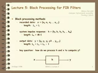
h Lecture 5: Block Processing for FIR Filters • Block processing methods • recorded data: x = {x0 x1 x2 … xL-1} • length: Lx = L • system impulse response: h = {h0 h1 h2 h3 … hM} • length: Lh = M+1 • output data: y = {y0 y1 y2 y3 … yLy-1} • length: Ly = Lx + Lh - 1 • key question: how do we process h and x to compute y? x y EE421, Lecture 5
Block Processing • Convolution tabley(0) = h(0)x(0)y(1) = h(0)x(1) + h(1)x(0)y(2) = h(0)x(2) + h(1)x(1) + h(2)x(0)y(3) = h(0)x(3) + h(1)x(2) + h(2)x(1) + h(3)x(0)y(4) = h(0)x(4) + h(1)x(3) + h(2)x(2) + h(3)x(1) + h(4)x(0) y(0) y(1) y(2) y(3) EE421, Lecture 5 y(4)
Block Processing • Convolution table • example: x = {1 2 1 3}, h = {4 2 1} n=0 n=0 y(0) = 4 y(1) = 10 y(2) = 9 y(3) = 16 y(4) = 7 y(5) = 3 y = {4 10 9 16 7 3} n=0 EE421, Lecture 5
Block Processing • LTI Formy(n) = … + x(0)h(n) + x(1)h(n-1) + x(2)h(n-2) + x(3)h(n-3) + … y(0) y(1) y(2) y(3) y(4) EE421, Lecture 5
Block Processing • LTI form • example: x = {1 2 1 3}, h = {4 2 1} n=0 n=0 4 10 9 16 7 3 0 y = {4 10 9 16 7 3} n=0 EE421, Lecture 5
Block Processing • Matrix form: EE421, Lecture 5
Block Processing • Matrix form • example: x = {1 2 1 3}, h = {4 2 1} n=0 n=0 y = {4 10 9 16 7 3} n=0 EE421, Lecture 5
h(2) h(1) h(0) h(2) h(1) h(0) h(2) h(1) h(0) h(2) h(1) h(0) h(2) h(1) h(0) h(2) h(1) h(0) y(0) y(1) y(2) y(3) y(4) y(5) Block Processing • Flip-and-slide form:y(n) = h(0)x(n) + h(1)x(n-1) + h(2)x(n-2) + … + h(L)x(n-L) EE421, Lecture 5
1 2 4 1 2 4 1 2 4 1 2 4 1 2 4 1 2 4 4 10 9 16 7 3 Block Processing • Flip-and-slide form: • example: x = {1 2 1 3}, h = {4 2 1} n=0 n=0 y = {4 10 9 16 7 3} n=0 EE421, Lecture 5
Block Processing • Programming considerations • convolution table formfunction y = conv(h, x) Lh = length(h);Lx = length(x);Ly = Lh+Lx-1;y = zeros(1,Ly);for n = 0:Ly-1 y(n+1) = 0; for i = 0:Lh-1 for j = 0:Lx-1 if (i+j == n) y(n+1) = y(n+1) + h(i+1)*x(j+1); end; end endend All these for loops will be inefficient in Matlab! EE421, Lecture 5
Block Processing • Programming considerations • LTI formfunction y = conv(h, x)Lh = length(h);Lx = length(x);Ly = Lh+Lx-1; y = zeros(1,Ly); for j = 0:Lx-1 shifth = [zeros(1, j) h zeros(1,Ly-Lh-j)]; y = y + x(j+1)*shifth;end Only 1 for loop! EE421, Lecture 5