Understanding Relationships Between Variables: ANOVA and Chi-Square Methods
This class focuses on the relationship between variables, emphasizing how social scientists analyze associations between qualitative and quantitative data. We cover two primary statistical methods: ANOVA (Analysis of Variance) and the Chi-square independence test. ANOVA assesses whether group means differ significantly, while the Chi-square test evaluates the independence of two qualitative variables. Students will learn to set hypotheses, interpret results, and apply these methods using statistical software like SPSS, gaining essential skills for analyzing data in various fields.


Understanding Relationships Between Variables: ANOVA and Chi-Square Methods
E N D
Presentation Transcript
CERAM February-March-April 2008 Class 3Relationship Between Variables Lionel Nesta Observatoire Français des Conjonctures Economiques Lionel.nesta@ofce.sciences-po.fr
Introduction • Typically, the social scientist is less interested in describing one variable than in describing the association between two or more variables. This class is devoted to the study of whether (yes or no) two variables are related (associated). • By relationship between variables, we mean any association between two dimensions, qualitative or quantitative or both, which appears to be systematic in some ways.
Structure of the Class • One qualitative (multinomial) and one quantitative (continuous/discrete) variables • Analysis of variance • Two qualitative (multinomial) variables • Chi-square (χ²) independence test • Two quantitative (continuous/discrete) variables • Correlation coefficient
ANOVA: ANalysis Of VAriance • ANOVA is a generalization of Student t test • Student test applies to two categories only: • H0: μ1 = μ2 • H1: μ1≠ μ2 • ANOVA is a method to test whether group means are equal or not. • H0: μ1 = μ2 = μ3 = ... = μn • H1: At least one mean differs significantly
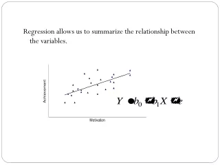
ANOVA This method is called after the fact that it is based on measures of variance. The F-statistics is a ratio comparing the variance due to group differences (explained variance) with the variance due to other phenomena (unexplained variance). Higher F means more explanatory power, thus more significance of groups.
Revenues (in million of US $ ) Do sectors differ significantly in their revenues? H0 : μ1 = μ2 = μ3 = ... = μn H1: At least one mean differs significantly.
residual df = (k – 1) df = n – k df = n – 1 ANOVA This decomposition produces Fisher’s Statistics as follows:
The ANOVA decomposition on Revenues The result tells me that I can reject the null Hypothesis H0 with 0.03% chances of rejecting the null Hypothesis H0 while H0 holds true (being wrong). I WILL TAKE THE CHANCE!!!
SPSS Application: ANOVA • Verify that US companies are larger than those from the rest of the world with an ANOVA • Are there systematic • Sectoral differences in terms of labour; R&D, sales • Write out H0 and H1for each variables • Analyse Comparer les moyennes ANOVA à un fateur • What do you conclude at 5% level? • What do you conclude at 1% level?
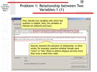
Introduction to Chi-Square • This part devoted to the study of whether two qualitative (categorical) variables are independent: H0: Independent:the two qualitative variables do not exhibit any systematic association. H1: Dependent: the category of one qualitative variable is associated with the category of another qualitative variable in some systematic way which departs significantly from randomness.
The Four Steps Towards The Test • Build the cross tabulation to compute observed joint frequencies • Compute expected joint frequencies under the assumption of independence • Compute the Chi-square (χ²) distance between observed and expected joint frequencies • Compute the significance of the χ²distance and conclude on H0 and H1
1. Cross Tabulation • A cross tabulation displays the joint distribution of two or more variables. They are usually referred to as a contingency tables. • A contingency table describes the distribution of two (or more) variables simultaneously. Each cell shows the number of respondents that gave a specific combination of responses, that is, each cell contains a single cross tabulation.
1. Cross Tabulation • We have data on two qualitative and categorical dimensions and we wish to know whether they are related • Region (AM, ASIA, EUR) • Type of company (DBF, LDF)
1. Cross Tabulation • We have data on two qualitative and categorical dimensions and we wish to know whether they are related • Region (AM, ASIA, EUR) • Type of company (DBF, LDF) AnalyseStatistiques descriptivesEffectifs
1. Cross Tabulation • We have data on two qualitative and categorical dimensions and we wish to know whether they are related • Region (AM, ASIA, EUR) • Type of company (DBF, LDF) AnalyseStatistiques descriptivesEffectifs
1. Cross Tabulation • Crossing Region (AM, ASIA, EUR) × Type of company (DBF, LDF) • AnalyseStatistiques descriptivesTableaux CroisésCelluleObservé
2. Expected Joint Frequencies • In order to say something on the relationship between two categorical variables, it would be nice to produce expected, also called theoretical, frequencies under the assumption of independence between the two variables.
2. Expected Joint Frequencies • Crossing Region (AM, ASIA, EUR) × Type of company (DBF, LDF) • AnalyseStatistiques descriptivesTableaux CroisésCelluleThéorique
2. Expected Joint Frequencies • AnalyseStatistiques descriptivesTableaux CroisésCelluleObservé & Théorique
3. Computing the χ² statistics • We can now compare what we observe with what we should observe, would the two variables be independent. The larger the difference, the less independent the two variables. This difference is termed a Chi-Square distance. With a contingency table ofn lines and m columns, the statistics follows a χ²distribution with (n-1)×(m-1) degree of freedom, with the lowest expected frequency being at least 5.
3. Computing the χ² statistics • AnalyseStatistiques descriptivesTableaux CroisésStatistiqueChi-deux
4. Conclusion on H0 versus H1 • We reject H0 with 0.00% chances of being wrong • I will take the chance, and I tentatively conclude that the type of companies and the regional origins are not independent. • Using our appreciative knowledge on biotechnology, it makes sense: biotechnology was first born in the USA, with European companies following and Asian (i.e. Japanese) companies being mainly large pharmaceutical companies. • Most DBFs are found in the US, then in Europe. This is less true now.
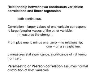
Introduction to Correlations • This part is devoted to the study of whether–and the extent to which– two or more quantitative variables are related: Positively correlated: the values of one variable “varying somewhat in step” with the values of another variable Negatively correlated: the values of one continuous variable “varying somewhat in opposite step” with the values of another variable Not correlated:the values of one continuous variable “varying randomly” when the values of another variable vary.
Pearson’s Linear Correlation Coefficient r • The Pearson product-moment correlation coefficient is a measure of the co-relation between two variables x and y. • Pearson's r reflects the intensity of linear relationship between two variables. It ranges from +1 to -1. • r near 1 : Positive Correlation • r near -1 : Positive Correlation • r near 0 :No or poor correlation
Pearson’s Linear Correlation Coefficient r Cov(x,y) : Covariance between x and y x et y : Standard deviation of x and Standard deviation of y n : Number of observations
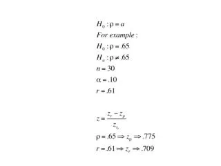
Pearson’s Linear Correlation Coefficient r • Is significantly different from 0 ? • H0 : rx,y= 0 • H1: rx,y 0 t* : if t* > t with (n – 2) degree of freedom and critical probability α (5%), we reject H0 and conclude that r significantly different from 0.
Pearson’s Linear Correlation Coefficient r • Analyse Corrélation Bivariée • Click on Pearson
Pearson’s Linear Correlation Coefficient r • Assumptions of Pearson’s r • There is a linear relationships between x and y • Both x and y are continuous random variables • Both variables are normally distributed • Equal differences between measurements represent equivalent intervals. We may want to relax (one of) these assumptions
Spearman’s Rank Correlation Coefficient ρ • Spearman's rank correlation is a non parametric measure of the intensity of a correlation between two variables, without making any assumptions about the distribution of the variables, i.e. about the linearity, normality or scale of the relationship. • near 1 : Positive Correlation • near -1 : Positive Correlation • near 0 : No or poor correlation
Spearman’s Rank Correlation Coefficient ρ d² : the difference between ranks of paired values of x and y n : Number of observations • ρ is simply a special case of the Pearson product-moment coefficient in which the data are converted to rankings before calculating the coefficient.
Spearman’s Rank Correlation Coefficient ρ • Analyse Corrélation Bivariée • Click on “Spearman”
Pearson’s r or Spearman’s ρ? • Relationship between tastes and levels of consumption on a large sample? (ρ) • Relationship between income and Consumption on a large sample? (r) • Relationship between income and Consumption on a small sample? Both (ρ) and (r)
Assignments on CERAM_LMC • Produce descriptive statistics on R&D, sales and number of employees, by sector • Perform an ANOVA to test whether there are significant differences between sectors in these three variables • Perform an ANOVA using the log of these three variables. What do you observe • Is the sector composition of the LMCs region specific?