Download
1 / 71
710 likes | 840 Vues
Lecture 2: Review of Instruction Sets, Pipelines, and Caches. Prof. David A. Patterson. Review, #1. Designing to Last through Trends Capacity Speed Logic 2x in 3 years 2x in 3 years DRAM 4x in 3 years 2x in 10 years Disk 4x in 3 years 2x in 10 years

E N D
Lecture 2: Review of Instruction Sets, Pipelines, and Caches Prof. David A. Patterson
Review, #1 • Designing to Last through Trends • Capacity Speed • Logic 2x in 3 years 2x in 3 years • DRAM 4x in 3 years 2x in 10 years • Disk 4x in 3 years 2x in 10 years • Processor ( n.a.) 2x in 1.5 years • Time to run the task • Execution time, response time, latency • Tasks per day, hour, week, sec, ns, … • Throughput, bandwidth • “X is n times faster than Y” means • ExTime(Y) Performance(X) • --------- = -------------- • ExTime(X) Performance(Y)
1 ExTimeold ExTimenew Speedupoverall = = (1 - Fractionenhanced) + Fractionenhanced Speedupenhanced Review, #2 • Amdahl’s Law: • CPI Law: • Execution time is the REAL measure of computer performance! • Good products created when have: • Good benchmarks • Good ways to summarize performance • Die Cost goes roughly with die area4 CPU time = Seconds = Instructions x Cycles x Seconds Program Program Instruction Cycle
Computer Architecture Is … the attributes of a [computing] system as seen by the programmer, i.e., the conceptual structure and functional behavior, as distinct from the organization of the data flows and controls the logic design, and the physical implementation. Amdahl, Blaaw, and Brooks, 1964 SOFTWARE
Computer Architecture’s Changing Definition • 1950s to 1960s: Computer Architecture Course = Computer Arithmetic • 1970s to mid 1980s: Computer Architecture Course = Instruction Set Design, especially ISA appropriate for compilers • 1990s: Computer Architecture Course = Design of CPU, memory system, I/O system, Multiprocessors
Instruction Set Architecture (ISA) software instruction set hardware
Interface Design • A good interface: • Lasts through many implementations (portability, compatability) • Is used in many differeny ways (generality) • Provides convenient functionality to higher levels • Permits an efficient implementation at lower levels use time imp 1 Interface use imp 2 use imp 3
Evolution of Instruction Sets Single Accumulator (EDSAC 1950) Accumulator + Index Registers (Manchester Mark I, IBM 700 series 1953) Separation of Programming Model from Implementation High-level Language Based Concept of a Family (B5000 1963) (IBM 360 1964) General Purpose Register Machines Complex Instruction Sets Load/Store Architecture (CDC 6600, Cray 1 1963-76) (Vax, Intel 432 1977-80) RISC (Mips,Sparc,HP-PA,IBM RS6000,PowerPC . . .1987) LIW/”EPIC”? (IA-64. . .1999)
Evolution of Instruction Sets • Major advances in computer architecture are typically associated with landmark instruction set designs • Ex: Stack vs GPR (System 360) • Design decisions must take into account: • technology • machine organization • programming langauges • compiler technology • operating systems • And they in turn influence these
A "Typical" RISC • 32-bit fixed format instruction (3 formats) • 32 32-bit GPR (R0 contains zero, DP take pair) • 3-address, reg-reg arithmetic instruction • Single address mode for load/store: base + displacement • no indirection • Simple branch conditions • Delayed branch see: SPARC, MIPS, HP PA-Risc, DEC Alpha, IBM PowerPC, CDC 6600, CDC 7600, Cray-1, Cray-2, Cray-3
Example: MIPS ( DLX) Register-Register 6 5 11 10 31 26 25 21 20 16 15 0 Op Rs1 Rs2 Rd Opx Register-Immediate 31 26 25 21 20 16 15 0 immediate Op Rs1 Rd Branch 31 26 25 21 20 16 15 0 immediate Op Rs1 Rs2/Opx Jump / Call 31 26 25 0 target Op
A B C D Pipelining: Its Natural! • Laundry Example • Ann, Brian, Cathy, Dave each have one load of clothes to wash, dry, and fold • Washer takes 30 minutes • Dryer takes 40 minutes • “Folder” takes 20 minutes
A B C D Sequential Laundry 6 PM Midnight 7 8 9 11 10 Time • Sequential laundry takes 6 hours for 4 loads • If they learned pipelining, how long would laundry take? 30 40 20 30 40 20 30 40 20 30 40 20 T a s k O r d e r
30 40 40 40 40 20 A B C D Pipelined LaundryStart work ASAP 6 PM Midnight 7 8 9 11 10 • Pipelined laundry takes 3.5 hours for 4 loads Time T a s k O r d e r
30 40 40 40 40 20 A B C D Pipelining Lessons 6 PM 7 8 9 • Pipelining doesn’t help latency of single task, it helps throughput of entire workload • Pipeline rate limited by slowest pipeline stage • Multiple tasks operating simultaneously • Potential speedup = Number pipe stages • Unbalanced lengths of pipe stages reduces speedup • Time to “fill” pipeline and time to “drain” it reduces speedup Time T a s k O r d e r
Computer Pipelines • Execute billions of instructions, so throughout is what matters • DLX desirable features: all instructions same length, registers located in same place in instruction format, memory operands only in loads or stores
5 Steps of DLX DatapathFigure 3.1, Page 130 Instruction Fetch Instr. Decode Reg. Fetch Execute Addr. Calc Memory Access Write Back IR L M D
Pipelined DLX DatapathFigure 3.4, page 137 Instruction Fetch Instr. Decode Reg. Fetch Execute Addr. Calc. Write Back Memory Access • Data stationary control • local decode for each instruction phase / pipeline stage
Visualizing PipeliningFigure 3.3, Page 133 Time (clock cycles) I n s t r. O r d e r
Its Not That Easy for Computers • Limits to pipelining: Hazards prevent next instruction from executing during its designated clock cycle • Structural hazards: HW cannot support this combination of instructions (single person to fold and put clothes away) • Data hazards: Instruction depends on result of prior instruction still in the pipeline (missing sock) • Control hazards: Pipelining of branches & other instructions • Common solution is to stall the pipeline until the hazardbubbles” in the pipeline
One Memory Port/Structural HazardsFigure 3.6, Page 142 Time (clock cycles) Load I n s t r. O r d e r Instr 1 Instr 2 Instr 3 Instr 4
One Memory Port/Structural HazardsFigure 3.7, Page 143 Time (clock cycles) Load I n s t r. O r d e r Instr 1 Instr 2 stall Instr 3
Speed Up Equation for Pipelining CPIpipelined = Ideal CPI + Pipeline stall clock cycles per instr Speedup = Ideal CPI x Pipeline depth Clock Cycleunpipelined Ideal CPI + Pipeline stall CPI Clock Cyclepipelined Speedup = Pipeline depth Clock Cycleunpipelined 1 + Pipeline stall CPI Clock Cyclepipelined x x
Example: Dual-port vs. Single-port • Machine A: Dual ported memory • Machine B: Single ported memory, but its pipelined implementation has a 1.05 times faster clock rate • Ideal CPI = 1 for both • Loads are 40% of instructions executed SpeedUpA = Pipeline Depth/(1 + 0) x (clockunpipe/clockpipe) = Pipeline Depth SpeedUpB = Pipeline Depth/(1 + 0.4 x 1) x (clockunpipe/(clockunpipe / 1.05) = (Pipeline Depth/1.4) x 1.05 = 0.75 x Pipeline Depth SpeedUpA / SpeedUpB = Pipeline Depth/(0.75 x Pipeline Depth) = 1.33 • Machine A is 1.33 times faster
Data Hazard on R1Figure 3.9, page 147 Time (clock cycles) IF ID/RF EX MEM WB I n s t r. O r d e r add r1,r2,r3 sub r4,r1,r3 and r6,r1,r7 or r8,r1,r9 xor r10,r1,r11
Three Generic Data Hazards InstrI followed by InstrJ • Read After Write (RAW)InstrJ tries to read operand before InstrI writes it
Three Generic Data Hazards InstrI followed by InstrJ • Write After Read (WAR)InstrJ tries to write operand before InstrI reads i • Gets wrong operand • Can’t happen in DLX 5 stage pipeline because: • All instructions take 5 stages, and • Reads are always in stage 2, and • Writes are always in stage 5
Three Generic Data Hazards InstrI followed by InstrJ • Write After Write (WAW)InstrJ tries to write operand before InstrI writes it • Leaves wrong result ( InstrI not InstrJ ) • Can’t happen in DLX 5 stage pipeline because: • All instructions take 5 stages, and • Writes are always in stage 5 • Will see WAR and WAW in later more complicated pipes
Forwarding to Avoid Data HazardFigure 3.10, Page 149 Time (clock cycles) I n s t r. O r d e r add r1,r2,r3 sub r4,r1,r3 and r6,r1,r7 or r8,r1,r9 xor r10,r1,r11
Data Hazard Even with ForwardingFigure 3.12, Page 153 Time (clock cycles) lwr1, 0(r2) I n s t r. O r d e r sub r4,r1,r6 and r6,r1,r7 or r8,r1,r9
Data Hazard Even with ForwardingFigure 3.13, Page 154 Time (clock cycles) I n s t r. O r d e r lwr1, 0(r2) sub r4,r1,r6 and r6,r1,r7 or r8,r1,r9
Software Scheduling to Avoid Load Hazards Try producing fast code for a = b + c; d = e – f; assuming a, b, c, d ,e, and f in memory. Slow code: LW Rb,b LW Rc,c ADD Ra,Rb,Rc SW a,Ra LW Re,e LW Rf,f SUB Rd,Re,Rf SW d,Rd Fast code: LW Rb,b LW Rc,c LW Re,e ADD Ra,Rb,Rc LW Rf,f SW a,Ra SUB Rd,Re,Rf SW d,Rd
Branch Stall Impact • If CPI = 1, 30% branch, Stall 3 cycles => new CPI = 1.9! • Two part solution: • Determine branch taken or not sooner, AND • Compute taken branch address earlier • DLX branch tests if register = 0 or ° 0 • DLX Solution: • Move Zero test to ID/RF stage • Adder to calculate new PC in ID/RF stage • 1 clock cycle penalty for branch versus 3
Pipelined DLX DatapathFigure 3.22, page 163 Instruction Fetch Instr. Decode Reg. Fetch Execute Addr. Calc. Memory Access Write Back This is the correct 1 cycle latency implementation!
Four Branch Hazard Alternatives #1: Stall until branch direction is clear #2: Predict Branch Not Taken • Execute successor instructions in sequence • “Squash” instructions in pipeline if branch actually taken • Advantage of late pipeline state update • 47% DLX branches not taken on average • PC+4 already calculated, so use it to get next instruction #3: Predict Branch Taken • 53% DLX branches taken on average • But haven’t calculated branch target address in DLX • DLX still incurs 1 cycle branch penalty • Other machines: branch target known before outcome
Four Branch Hazard Alternatives #4: Delayed Branch • Define branch to take place AFTER a following instruction branch instruction sequential successor1 sequential successor2 ........ sequential successorn branch target if taken • 1 slot delay allows proper decision and branch target address in 5 stage pipeline • DLX uses this Branch delay of length n
Delayed Branch • Where to get instructions to fill branch delay slot? • Before branch instruction • From the target address: only valuable when branch taken • From fall through: only valuable when branch not taken • Cancelling branches allow more slots to be filled • Compiler effectiveness for single branch delay slot: • Fills about 60% of branch delay slots • About 80% of instructions executed in branch delay slots useful in computation • About 50% (60% x 80%) of slots usefully filled • Delayed Branch downside: 7-8 stage pipelines, multiple instructions issued per clock (superscalar)
Evaluating Branch Alternatives Scheduling Branch CPI speedup v. speedup v. scheme penalty unpipelined stall Stall pipeline 3 1.42 3.5 1.0 Predict taken 1 1.14 4.4 1.26 Predict not taken 1 1.09 4.5 1.29 Delayed branch 0.5 1.07 4.6 1.31 Conditional & Unconditional = 14%, 65% change PC
Pipelining Introduction Summary • Just overlap tasks, and easy if tasks are independent • Speed Up Pipeline Depth; if ideal CPI is 1, then: • Hazards limit performance on computers: • Structural: need more HW resources • Data (RAW,WAR,WAW): need forwarding, compiler scheduling • Control: delayed branch, prediction Pipeline Depth Clock Cycle Unpipelined Speedup = X Clock Cycle Pipelined 1 + Pipeline stall CPI
Recap: Who Cares About the Memory Hierarchy? Processor-DRAM Memory Gap (latency) µProc 60%/yr. (2X/1.5yr) 1000 CPU “Moore’s Law” 100 Processor-Memory Performance Gap:(grows 50% / year) Performance 10 DRAM 9%/yr. (2X/10 yrs) DRAM 1 1980 1981 1982 1983 1984 1985 1986 1987 1988 1989 1990 1991 1992 1993 1994 1995 1996 1997 1998 1999 2000 Time
Levels of the Memory Hierarchy Upper Level Capacity Access Time Cost Staging Xfer Unit faster CPU Registers 100s Bytes <10s ns Registers prog./compiler 1-8 bytes Instr. Operands Cache K Bytes 10-100 ns 1-0.1 cents/bit Cache cache cntl 8-128 bytes Blocks Main Memory M Bytes 200ns- 500ns $.0001-.00001 cents /bit Memory OS 512-4K bytes Pages Disk G Bytes, 10 ms (10,000,000 ns) 10 - 10 cents/bit Disk -6 -5 user/operator Mbytes Files Larger Tape infinite sec-min 10 Tape Lower Level -8
The Principle of Locality • The Principle of Locality: • Program access a relatively small portion of the address space at any instant of time. • Two Different Types of Locality: • Temporal Locality (Locality in Time): If an item is referenced, it will tend to be referenced again soon (e.g., loops, reuse) • Spatial Locality (Locality in Space): If an item is referenced, items whose addresses are close by tend to be referenced soon (e.g., straightline code, array access) • Last 15 years, HW relied on localilty for speed
Memory Hierarchy: Terminology • Hit: data appears in some block in the upper level (example: Block X) • Hit Rate: the fraction of memory access found in the upper level • Hit Time: Time to access the upper level which consists of RAM access time + Time to determine hit/miss • Miss: data needs to be retrieve from a block in the lower level (Block Y) • Miss Rate = 1 - (Hit Rate) • Miss Penalty: Time to replace a block in the upper level + Time to deliver the block the processor • Hit Time << Miss Penalty (500 instructions on 21264!) Lower Level Memory Upper Level Memory To Processor Blk X From Processor Blk Y
Cache Measures • Hit rate: fraction found in that level • So high that usually talk about Miss rate • Miss rate fallacy: as MIPS to CPU performance, miss rate to average memory access time in memory • Average memory-access time = Hit time + Miss rate x Miss penalty (ns or clocks) • Miss penalty: time to replace a block from lower level, including time to replace in CPU • access time: time to lower level = f(latency to lower level) • transfer time: time to transfer block =f(BW between upper & lower levels)
Simplest Cache: Direct Mapped Memory Address Memory 0 4 Byte Direct Mapped Cache 1 Cache Index 2 • Location 0 can be occupied by data from: • Memory location 0, 4, 8, ... etc. • In general: any memory locationwhose 2 LSBs of the address are 0s • Address<1:0> => cache index • Which one should we place in the cache? • How can we tell which one is in the cache? 0 3 1 4 2 5 3 6 7 8 9 A B C D E F
1 KB Direct Mapped Cache, 32B blocks • For a 2 ** N byte cache: • The uppermost (32 - N) bits are always the Cache Tag • The lowest M bits are the Byte Select (Block Size = 2 ** M) 31 9 4 0 Cache Tag Example: 0x50 Cache Index Byte Select Ex: 0x01 Ex: 0x00 Stored as part of the cache “state” Valid Bit Cache Tag Cache Data : Byte 31 Byte 1 Byte 0 0 : 0x50 Byte 63 Byte 33 Byte 32 1 2 3 : : : : Byte 1023 Byte 992 31
Cache Data Cache Tag Valid Cache Block 0 : : : Compare Two-way Set Associative Cache • N-way set associative: N entries for each Cache Index • N direct mapped caches operates in parallel (N typically 2 to 4) • Example: Two-way set associative cache • Cache Index selects a “set” from the cache • The two tags in the set are compared in parallel • Data is selected based on the tag result Cache Index Valid Cache Tag Cache Data Cache Block 0 : : : Adr Tag Compare 1 0 Mux Sel1 Sel0 OR Cache Block Hit