Between Competition and Monopoly
7. Between Competition and Monopoly. Outline. Monopolistic Competition Oligopoly Monopolistic Competition, Oligopoly, and Public Welfare A Glance Backward: Comparing the Four Market Forms. Three Real World Puzzles. Why are there so many retailers?

Between Competition and Monopoly
E N D
Presentation Transcript
7 Between Competition and Monopoly
Outline • Monopolistic Competition • Oligopoly • Monopolistic Competition, Oligopoly, and Public Welfare • A Glance Backward: Comparing the Four Market Forms
Three Real World Puzzles • Why are there so many retailers? • E.g., intersections with 4 gas stations which is more than # of cars warrants. Why and how do they all stay open? • Why do oligopolists advertise more than competitive firms? • E.g., many big Co. use ads to battle for customers and ad budgets account for a huge portion of TC. Vs. farmers where few if any farms spend $ on ads. • Why do oligopolists seem to ∆P so infrequently? • E.g., ∆P commodities hourly but ∆P cars or refrigerators only a few times a year.
Characteristics of Monopolistic Competition • Many small buyers and sellers • Freedom of entry and exit • Perfect information • Heterogeneous products: each seller’s product differs somewhat from every other seller’s product. • E.g., Diff. in packaging, services, or consumers’ perceptions. • Only characteristic that differs from perfect competition.
Monopolistic Competition • D curve facing firm has (-) slope. • Each seller’s product is different –they are not perfect substitutes. • ↑P will drive away some but not all of firm’s customers. Or ↓P will attract some but not all customers from rival firms. • Freedom of entry and exit → firms cannot earn econ Π in LR. • SR Π > 0 → new firms enter and ↓P until P = AC. • Most U.S. firms are in this market structure.
Determination of Price and Output under Monopolistic Competition • Recall when D has (-) slope → P > MR. • Profit-max Q is where MR = MC. • Analysis looks like pure monopoly, but monop. comp. firm (with rivals producing close substitutes) has a much flatter D curve. • LR: Π = 0 → each firm produces where P = AC. So firm’s D curve must be tangent to its AC curve. • Zero econ. Π in LR is seen in real world. • E.g., Gas station owners do not earn higher Π than small farmers under perfect competition.
MC AC P C E D MR FIGURE 1. Short-Run Equilibrium Under Monopolistic Competition Π-max Q =12,000 and P = $3.50 Per unit Π= $0.10 → total Π = $1,200. $3.80 $3.50 Price per Gallon 3.40 $3.00 12,000 Gallons of Gasoline per Week
MC AC M P E D MR FIGURE 2.Long-Run Equilibrium Under Monopolistic Competition SR profits in Fig. 1 → new firms enter which shifts each firm’s D curve down until P = AC. Compared with SR profits in Fig. 1: a. P is lower in LR b. more firms in industry; each produces a smaller Q with higher AC. $3.45 $3.35 Price per Gallon 10,000 15,000 Gallons of Gasoline per Week
The Excess Capacity Theorem • In Fig. 2, AC at LR Q of firm (pt P) > min AC (pt M). • Pt M is where LR Q of a perf. comp. firm would be. • In LR, monop. comp. firm is producing where ↓AC but has not yet reached its min. • Monopolistic competition leads to firms that have unused or wasted capacity. • Resolve puzzle 1 –abundance of retailers: intersection with 4 gas stations where 2 would suffice and operate at lower AC is real world ex. of excess capacity.
The Excess Capacity Theorem • Fewer firms in a monop. comp. market → each firm could ↑Q and ↓AC. • Yet, fewer firms with larger quantities means there is less variety of product. • Greater efficiency would be achieved at the cost of greater standardization. • Not clear society would be better off with fewer firms.
Oligopoly Defined • Oligopoly = market dominated by a few sellers, where several are large enough to affect market P. • Great rivalry among firms with new product intros, free samples, and agro marketing campaigns. • Degree of product differentiation varies by industry: none in steel plates but lots in cars. • Some industries also contain large # of smaller firms (e.g., soft drinks) but they are dominated by a few large firms that get bulk of industry sales.
Oligopoly Defined • Firms strive to create unique products (in terms of features, location, or appeal) to shield themselves from competition that ↓P and ↓sales. • More intense competition than pure competition. • E.g., A corn farmer doesn’t make tough P decisions. He accepts market P and reacts by picking Q. • A farmer doesn’t need to advertise. He can sell as much as he likes at current market P. • A farmer doesn’t worry about P policies his rivals are planning.
Oligopoly Defined • Oligopolists have some influence over market P, so they must consider rivals’ P; spend a fortune on ads; and try to predict their rivals’ actions. • Resolve puzzle 2 –why oligopolists advertise and perfectly competitive firms do not. • Comp. firms can sell as much as they want at current P, so why advertise? Vs. Toyota faces a (-) sloped D curve, so it must ↓P or ↑ads (try to shift D out) to sell more cars. • Products are identical, so farm A’s ads might ↑ sales of farm B. Vs. Toyota’s ads may ↑ its sales and ↓ sales of rival carmakers.
Why Oligopolistic Behavior is So Difficult to Analyze • Largest firms can impact P and all firms must watch rivals’ actions. • Analysis is difficult as firms’ decisions are inter-dependent and oligopolists know that outcomes of their decisions depend on rivals’ responses. • E.g., Toyota’s managers know that their actions will cause reactions by Honda which may require Toyota to adjust its plans. • Oligopolies have a variety of behavior patterns which requires different models to understand their behavior.
Models of Oligopoly • Different models to understand Oligopoly behavior: • Ignore interdependence • Strategic interaction • Cartels • Price leadership and tacit collusion • Sales maximization • Kinked demand curve • Game theory
Ignoring Interdependence • Simplest model • Firms behave as if their actions will not spark reactions from rivals. • Each firm seeks to max profits and assumes its P-Q decision will not affect its rivals’ strategy. • Analyze oligopoly in the same way as pure monopoly. • This doesn’t explain most oligopoly behavior!
Strategic Interaction • Consider 2 soap makers: X and Y. • X ↓P to $4.05 and assumes Y will continue its P = $4.12 • Say Qx = 5m and X spends $1m on ads. • X may be surprised when Y cuts P to $4.00; ↑Qy to 8m and sponsors the Super Bowl. • This ↓Πx and X wishes it didn’t cut P in first place. • X cannot afford to ignore how Y will react.
Cartels • All firms agree to set P and Q → act as pure monopolist. • OPEC began making joint decisions in 1970’s and has been successful over time at ↓Q oil and ↑P oil. • Cartels are difficult to organize and hard to enforce. • Each member must produce small Q assigned by group. But once high P is established, every firm is tempted to cheat by ↑Qs. When cheating is suspected, cartel quickly falls apart as others ↑Qs which ↓P. • Considered worse than monopoly. Cartel charges monopoly P without the cost savings from large scale production.
Price Leadership and Tacit Collusion • Overt collusion (where firms meet to pick P-Q) is illegal in the U.S. and rare. But tacit collusion is common. • Each tacitly colluding firm hopes that if it does not rock the boat (via ↓P or ↑ads), then rivals will do same. • Price leadership = 1 firm makes P decisions for group. • Other firms are expected to adopt P of leader without any explicit agreement. • P leader is often largest firm in industry.
Sales Maximization: Model with Interdependence Ignored • Firms may attempt to max revenue rather than profit if: • control is separated from ownership • compensation of managers is related to size of the firm • Q set where MR = 0 (rather than MR = MC) • Recall: MR is slope of TR curve. So TR is max when MR = 0. If MR > 0 → ↑Q to ↑TR and if MR < 0 → ↓Q to ↑TR. • Compared to profit-max firm: • Higher Q • Lower P
MC AC E F A D B MR FIGURE 3.Sales-Max Equilibrium Π-max Q = 2.5m where MR = MC. P = $4.00 and total Π = $0.20 x 2.5 m = $500,000. Sales-max Q = 3.75m where MR = 0. P = $3.75 and totalΠ= $0.06 x 3.75 m = $225,000. TotalΠ(TR) is lower (higher) at point F than point E. $4.00 3.80 Price per Box 3.75 3.69 2.5 3.75 Millions of Boxes per Year
? The Kinked Demand Curve Model • Resolve puzzle 3 –why do P in oligopolistic markets (cars or appliances) change less often than P of commodities (wheat or gold)? • Firms think that other firms will match any P cut, but not any P increase. If true, firms face an inelastic D curve with P cuts and an elastic curve with P increases.
? The Kinked Demand Curve Model • In Fig. 4, pt A is firm’s initial P = $8. • 2 D curves pass through pt A. • DD is more elastic → rivals’ P are fixed • dd is less elastic → rivals match ∆P • If firm ↓P to $7 (and rivals don’t match ↓P) → large ↑customers, so new Qd = 1,400. • If rivals match ↓P → ↑Qd is small, so new Qd = 1,100. • If firm ↑P (and rivals don’t match ↑P) → large ↓Qd.
? The Kinked Demand Curve Model • The firm’s true demand curve in Fig. 4 is DAd –a kinked demand curve. • P tend to “stick” to their original level because ↑P → lose many customers and ↓P → gain very few customers. • Firm will only ∆P if costs change enormously.
d D A (Competitors’ D prices are fixed) (Competitors respond to price d changes) FIGURE 4.The Kinked Demand Curve Typical oligopoly fears the worst. If firm cuts P then rivals will match P cut → relevant demand curve is dd. But if firm raises P then rival will not match the P increase → relevant demand curve is DD. Thus, the firm’s true demand curve is the red line “DAd.” Price $8 7 0 1,000 1,100 1,400 Quantity per Year
? The Kinked Demand Curve Model • MR is associated with DD and mr is associated with dd. • Overall marginal revenue curve is DBCmr. • MC = MR at pt E which shows Π-max Q for oligopolist. • Since relevant MR curve is kinked, even a moderate shift in MC will leave Q and thereby P unchanged. • Oligopoly prices are “sticky” and do not respond to minor cost changes.
d MC D A B D E MR d C mr FIGURE 5.The Kinked Demand Curve and Sticky Prices Price $8 1,000 Quantity Supplied per Year
The Game-Theory Approach • Most widely used approach to analyze oligopoly behavior. • Each oligopolist is seen as a competing player in a game of strategy. • Optimal strategies are determined by examining a payoff matrix showing Π of each firm depending on P strategy that each firm follows.
Games with Dominant Strategies • Dominant strategy = one that gives the bigger payoff to the firm that selects it, no matter which of the two strategies the competitor selects. • E.g., Table 1., both firms have an incentive to pick low P strategy regardless of what other firm does. If B picks high P, then A receives largest payoff choosing low P. Or if B picks low P, then A receives the largest payoff by choosing low P. • “Low Price” is the dominant strategy for both firms, so both charge a low P and each earns $3m.
TABLE 1.Payoff Matrix with Dominant Strategies Firm B Strategy High Price Low Price High Price Firm A Strategy Low Price
Games with Dominant Strategies • A market with a duopoly serves public interest better than a monopoly because of the competition created between two firms. • Both firms would be better off if they could charge high P. But the presence of a competitor, forces each firm to protect itself by charging low P. • It is damaging to the public to allow rival firms to collude on what prices to charge for their products. • E.g., if two firms collude in Table 1, then we end up with high P and each earning $10m.
Games without Dominant Strategies • Maximin = select the strategy that yields the max payoff assuming your rival does as much damage to you as he can. • In Table 2, A’s maximin strategy is to pick low P and earn $5m. • Firm A thinks: if I chose a high P → worst outcome is B picks a low P and I get $3m. If I chose a low P → worst outcome is B picks a low P and I get $5m. • Firm A picks the strategy that offers the best of those bad outcomes.
TABLE 2.A Payoff Matrix without a Dominant Strategy Firm B Strategy High Price Low Price High Price Firm A Strategy Low Price
Repeated Games • Repeated games give players the opportunity to learn something about each other’s behavior patterns and, perhaps, to arrive at mutually beneficial arrangements. • Table 1 shows a single round of the game. Each firm picked low P. But if games are repeated, players can escape this trap. • E.g., Firm A could cultivate a reputation of “tit for tat.” Each time B charges a high P → A would charge a high P. After a few repetitions, B learns that A always matches its P decisions. So B will see that it’s better to stick with a high P.
Threats and Credibility • Use threats to induce rivals to change their behavior. • E.g., retailer could threaten to double Q and ↓P to $0 if a rival imitates its product. But this is not credible, because it hurts the retailer who is making the threat. • A credible threat is a threat that does not harm the threatener if it is carried out. • Old firms often use credible threats to prevent new firms from entering the industry. • E.g., old firm will build a larger factory than it would otherwise want. Large factory lowers cost of ↑Q –even at low P.
Possible Choices Possible Reactions of Old Firm of New Firm –2 –2 Enter Don’t Enter Big Factory 4 0 2 2 Enter Small Factory Don’t Enter 6 0 FIGURE 6. Entry and Entry-Blocking Strategy Profits (millions $) Old Firm New Firm
Threats and Credibility • In Fig. 6, best outcome for old firm is to have a small factory and no rivals. • But if old firm builds a small factory, it can count on new firm entering to earn $2m. So old firm’s ↓Π to $2m. • If old firm builds a big factory, its ↑Q will ↓P and ↓Π. Old firm now earns $4m if new firm stays out. • Clearly, new firm will stay out to avoid loses of $2m. • Thus, old firm should build big factory to keep rivals out.
Monopolistic Competition, Oligopoly, & Public Welfare • Oligopolistic behavior is so varied that it is hard to come to a simple conclusion about welfare implications. • In many circumstances, the behavior of monopolistic competitors and oligopolists falls short of the social optimum. • Excess capacity theorem suggests monopolistic competition can lead to inefficiently high production costs. • Oligopolists may organize into successful cartels to ↓Q and ↑P.
Monopolistic Competition, Oligopoly, & Public Welfare • When an oligopolistic market is perfectly contestable –if firms can enter and exit without losing $ they invested –then (P,Q) of firms is likely to be socially efficient. • E.g., airplanes, trucks, and barges can easily be moved. • Constant threat of entry forces oligopolists to keep their prices down and their costs low.
Comparing the Four Market Forms • Perfect competition and pure monopoly are rare. • Most firms are monopolistically competitive, but oligopoly firms account for largest share of economy’s output. • Π = 0 in LR under perfect competition and monopolistic competition because of free entry and exit. • Thus, P = AC in LR under these 2 market forms. • Π-max firm under any market form selects Q by setting MR = MC. • However, oligopolists may not set MC = MR when choosing Q –e.g., if firm max sales.
Comparing the Four Market Forms • Perfectly competitive firm and industry efficient allocation of resources. • Monopoly inefficient allocation of resources by ↓Q and ↑P. • Monopolisticcompetition inefficient allocation of resources through excess capacity. • Under oligopoly, almost anything can happen, impossible to generalize about its vices or virtues.