Numerical solutions of equations
300 likes | 564 Vues
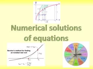
Numerical solutions of equations. Introduction. This chapter gives you several methods which can be used to solve complicated equations to given levels of accuracy These are similar to methods which computers and calculators will use, and hence can be used in computer programming.

Numerical solutions of equations
E N D
Presentation Transcript
Introduction • This chapter gives you several methods which can be used to solve complicated equations to given levels of accuracy • These are similar to methods which computers and calculators will use, and hence can be used in computer programming
Numerical solutions of equations You can solve equations of the form f(x) = 0 using interval bisection Interval bisection is a variation on Trial and Improvement which you will have seen at GCSE level Interval Bisection is an iterative process which allows us to find a root to whatever degree of accuracy we wish (usually 1-2 decimal places!) An iterative process is one which is a short set of instructions which are then repeated as many times as needed As a result such processes can be used in computers and calculators so they can solve equations 2A
Numerical solutions of equations You can solve equations of the form f(x) = 0 using interval bisection Use Interval Bisection to find √11 to 1 decimal place Set this up as an equation: Sub in integers until we find a change of sign Square both sides Subtract 11 So an solution lies between 3 and 4 2A
Numerical solutions of equations You can solve equations of the form f(x) = 0 using interval bisection Use Interval Bisection to find √11 to 1 decimal place So a solution lies between 3 and 4. • Now we set up a table, subbing these 2 values into f(x), as well as the midpoint of these • When you have found the midpoint and substituted it in, choose the positive and negative answers closest to 0 • The answer will be between these. Now repeat the process for these 2 numbers Our answer must be between 3.3125 and 3.34375 To one decimal place, the answer therefore must be 3.3! 2A
Numerical solutions of equations You can solve equations of the form f(x) = 0 using interval bisection Show that a root of the equation: lies between 0 and 1 Use interval bisection 4 times to find an approximation for this root Sub in 0 and 1 to show the sign of the answer changes As the sign has changed, a solution must lie between 0 and 1… 2A
Numerical solutions of equations You can solve equations of the form f(x) = 0 using interval bisection Show that a root of the equation: lies between 0 and 1 Use interval bisection 4 times to find an approximation for this root Our approximation is the final bisection 0.6875 (or round if necessary) 2A
Numerical solutions of equations You can solve equations of the form f(x) = 0 using linear interpolation In linear interpolation, you first draw a sketch of the function between 2 intervals Then, you draw a straight line between the interval coordinates (this will be a rough approximation to the curve You can then use similar triangles to find the place the straight line crosses the x-axis (the ‘root’ as it were) You then update the interval and repeat the process… 2B
Numerical solutions of equations You can solve equations of the form f(x) = 0 using linear interpolation A solution of the equation: lies in the interval [1,2]. Use linear interpolation to find this root, correct to one decimal place. Sub in 1 and 2 to show the sign of the answer changes As the sign has changed, a solution must lie between 1 and 2… 2B
Numerical solutions of equations y (2,7) You can solve equations of the form f(x) = 0 using linear interpolation A solution of the equation: lies in the interval [1,2]. Use linear interpolation to find this root, correct to one decimal place. x x (1,-4) • After sketching the graph between the limits, draw a straight line between them • The place this crosses the x-axis is an approximation for the root • You can call it x and then use similar triangles to find its value Now sketch the graph between x = 1 and x = 2 (the limits you were given) It does not have to be really accurate! 2B
Numerical solutions of equations y (2,7) You can solve equations of the form f(x) = 0 using linear interpolation A solution of the equation: lies in the interval [1,2]. Use linear interpolation to find this root, correct to one decimal place. 7 x-1 2-x x x 4 • Imagine creating triangles using the x-axis and the coordinates marked • Label the sides, using x as the place the straight line crosses the x-axis • These two triangles are similar – ie) They have the same angles (both have a right angle and two other pairs that are the same – you can see this from the vertically opposite angles at the centre and the ‘alternate’ angles ta the top and bottom!) • In similar triangles, a long side divided by a shorter side will give the same answer (provided that equivalent sides are used!) (1,-4) 2B
Numerical solutions of equations y (2,7) You can solve equations of the form f(x) = 0 using linear interpolation A solution of the equation: lies in the interval [1,2]. Use linear interpolation to find this root, correct to one decimal place. 7 x-1 2-x x x 4 Short side ÷ longer side in each triangle gives the same answer… (1,-4) Multiply the whole left by 7 and the whole right by 4 Multiply by 28 to leave the numerators Add 4x, Add 7 So the value of x is 15/11 or 1.3636… Divide by 11 2B
Numerical solutions of equations y (2,7) You can solve equations of the form f(x) = 0 using linear interpolation A solution of the equation: lies in the interval [1,2]. Use linear interpolation to find this root, correct to one decimal place. 7 15/11 x-1 2-x x x 4 • So the value of x is 15/11 or 1.3636… (15/11,-1.009….) (1,-4) Sub in 15/11 to find the value on the curve at this point Calculate • We now repeat the process from this new point… 2B
Numerical solutions of equations y (2,7) You can solve equations of the form f(x) = 0 using linear interpolation A solution of the equation: lies in the interval [1,2]. Use linear interpolation to find this root, correct to one decimal place. x x • As you can see, the new estimate for the root is closer than the first approximation • Repeat the process using these new values (strictly speaking the original estimate was x1, and this one is x2 – use this notation when you solve these problems!) (15/11,-1.009….) 2B
Numerical solutions of equations y (2,7) You can solve equations of the form f(x) = 0 using linear interpolation A solution of the equation: lies in the interval [1,2]. Use linear interpolation to find this root, correct to one decimal place. 7 x-15/11 2-x x x 1.009… (15/11,-1.009….) Cross-multiply Expand brackets • Repeat this process several times until your answer is accurate to the requested degree • Try to be as accurate as possible at each stage, avoiding rounding too much • Draw a new sketch at each stage • Use x1, x2, x3 to represent each approximation! Rearrange Solve 2B
Numerical solutions of equations You can solve equations of the form f(x) = 0 using the Newton-Raphson process The Newton-Raphson formula is as follows: The function we are solving, with our current approximation substituted in The derivative of the function we are solving, with our current approximation substituted in Our next approximation for the root Our current approximation for the root 2C
Numerical solutions of equations You can solve equations of the form f(x) = 0 using the Newton-Raphson process Use the Newton-Raphson process to find the root of the equation: Use x0 = 3 and give your answer to 2 decimal places. Find the function and its derivative first… Rearrange Differentiate 2C
Numerical solutions of equations You can solve equations of the form f(x) = 0 using the Newton-Raphson process Use the Newton-Raphson process to find the root of the equation: Use x0 = 3 and give your answer to 2 decimal places. Our current approximation is x0, replace the fraction with equivalent expressions Sub in x0 = 3 Calculate 2C
Numerical solutions of equations Repeat the process, but now we use the value of x1 to find x2 You can solve equations of the form f(x) = 0 using the Newton-Raphson process Use the Newton-Raphson process to find the root of the equation: Use x0 = 3 and give your answer to 2 decimal places. Sub in x1 = 2.912 Calculate As both x1 and x2 round to 2.91, then this is the solution to 2 decimal places! 2C
Numerical solutions of equations You can solve equations of the form f(x) = 0 using the Newton-Raphson process Use the Newton-Raphson process twice to find approximate a root of the equation: Use x0 = 2 as your first approximation and give your answer to 3 decimal places. Differentiate 2C
Numerical solutions of equations You can solve equations of the form f(x) = 0 using the Newton-Raphson process Use the Newton-Raphson process twice to find approximate a root of the equation: Use x0 = 2 as your first approximation and give your answer to 3 decimal places. Sub in x0 as our first approximation and replace the parts of the fraction Sub in x0 = 2 Calculate 2C
Numerical solutions of equations You can solve equations of the form f(x) = 0 using the Newton-Raphson process Use the Newton-Raphson process twice to find approximate a root of the equation: Use x0 = 2 as your first approximation and give your answer to 3 decimal places. Sub in x1 = 1.866 Calculate It is important to note that the Newton-Raphson method will not always work, sometimes tending away from a root rather than towards it Usually, choosing a different first approximation will correct this! 2C
Summary • You have learnt several iterative methods for solving equations • Although these may seem cumbersome, the ideas involved in these are used in computers and calculators • They will also work when other methods fail to find answers! 2C