Download
1 / 48
530 likes | 854 Vues
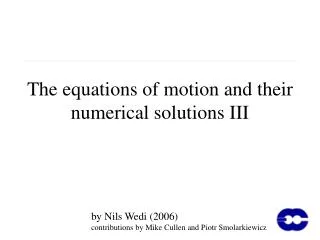
The equations of motion and their numerical solutions II. by Nils Wedi (2006) contributions by Mike Cullen and Piotr Smolarkiewicz. Dry “dynamical core” equations. Shallow water equations Isopycnic/isentropic equations Compressible Euler equations Incompressible Euler equations

E N D
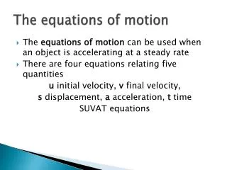
The equations of motion and their numerical solutions II by Nils Wedi (2006) contributions by Mike Cullen and Piotr Smolarkiewicz
Dry “dynamical core” equations • Shallow water equations • Isopycnic/isentropic equations • Compressible Euler equations • Incompressible Euler equations • Boussinesq-type approximations • Anelastic equations • Primitive equations • Pressure or mass coordinate equations
Shallow water equations eg. Gill (1982) Numerical implementation by transformation to a Generalized transport form for the momentum flux: This form can be solved by eg. MPDATA Smolarkiewicz and Margolin (1998)
Isopycnic/isentropic equations eg. Bleck (1974); Hsu and Arakawa (1990); isentropic isopycnic shallow water defines depth between “shallow water layers”
More general isentropic-sigma equations Konor and Arakawa (1997);
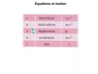
Euler equations for isentropic inviscid motion Speed of sound (in dry air 15ºC dry air ~ 340m/s)
Reference and environmental profiles Distinguish between • (only vertically varying) static reference or basic state profile (used to facilitate comprehension of the full equations) • Environmental or balanced state profile (used in general procedures to stabilize or increase the accuracy of numerical integrations; satisfies all or a subset of the full equations, more recently attempts to have a locally reconstructed hydrostatic balanced state or use a previous time step as the balanced state
The use of reference and environmental/balanced profiles • For reasons of numerical accuracy and/or stability an environmental/balanced state is often subtracted from the governing equations Clark and Farley (1984)
*NOT* approximated Euler perturbation equations eg. Durran (1999) using:
Incompressible Euler equations eg. Durran (1999); Casulli and Cheng (1992); Casulli (1998);
Example of simulation with sharp density gradient Animation: "two-layer" simulation of a critical flow past a gentle mountain Compare to shallow water: reduced domain simulation with H prescribed by an explicit shallow water model
Classical Boussinesq approximation eg. Durran (1999)
Projection method Subject to boundary conditions !!!
Integrability condition With boundary condition:
Solution Ap = f Since there is a discretization in space !!! Most commonly used techniques for the iterative solution of sparse linear-algebraic systems that arise in fluid dynamics are the preconditioned conjugate gradient method and the multigrid method. Durran (1999)
Importance of the Boussinesq linearization in the momentum equation Two layer flow animation with density ratio 1:1000 Equivalent to air-water Incompressible Euler two-layer fluid flow past obstacle Incompressible Boussinesq two-layer fluid flow past obstacle Two layer flow animation with density ratio 297:300 Equivalent to moist air [~ 17g/kg] - dry air Incompressible Euler two-layer fluid flow past obstacle Incompressible Boussinesq two-layer fluid flow past obstacle
Anelastic approximation Batchelor (1953); Ogura and Philipps (1962); Wilhelmson and Ogura (1972); Lipps and Hemler (1982); Bacmeister and Schoeberl (1989); Durran (1989); Bannon (1996);
Anelastic approximation Lipps and Hemler (1982);
Numerical Approximation Compact conservation-law form: Lagrangian Form:
Numerical Approximation with LE, flux-form Eulerian or Semi-Lagrangian formulation using MPDATA advection schemes Smolarkiewicz and Margolin (JCP, 1998) with Prusa and Smolarkiewicz (JCP, 2003) specified and/or periodic boundaries
Importance of implementation detail? Example of translating oscillator (Smolarkiewicz, 2005): time
Example ”Naive” centered-in-space-and-time discretization: Non-oscillatory forward in time (NFT) discretization: paraphrase of so called “Strang splitting”, Smolarkiewicz and Margolin (1993)
Compressible Euler equations Davies et al. (2003)
A semi-Lagrangian semi-implicit solution procedure (not as implemented, Davies et al. (2005) for details) Davies et al. (1998,2005)
A semi-Lagrangian semi-implicit solution procedure Non-constant- coefficient approach!
Pressure based formulationsHydrostatic Hydrostatic equations in pressure coordinates
Pressure based formulationsHistorical NH Miller (1974); Miller and White (1984);
Pressure based formulationsHirlam NH Rõõm et. Al (2001), and references therein;
Pressure based formulationsMass-coordinate Laprise (1992) Define ‘mass-based coordinate’ coordinate: ‘hydrostatic pressure’ in a vertically unbounded shallow atmosphere By definition monotonic with respect to geometrical height Relates toRõõm et. Al (2001):
Pressure based formulations Laprise (1992) Momentum equation Thermodynamic equation Continuity equation with
Pressure based formulationsECMWF/Arpege/Aladin NH model Bubnova et al. (1995); Benard et al. (2004), Benard (2004) hybrid vertical coordinate Simmons and Burridge (1981) coordinate transformation coefficient scaled pressure departure ‘vertical divergence’ with
Hydrostatic vs. Non-hydrostatic eg. Keller (1994) • Estimation of the validity
Hydrostatic vs. Non-hydrostatic Hydrostatic flow past a mountain without wind shear Non-hydrostatic flow past a mountain without wind shear
Hydrostatic vs. Non-hydrostatic Hydrostatic flow past a mountain with vertical wind shear Non-hydrostatic flow past a mountain with vertical wind shear But still fairly high resolution L ~ 30-100 km
Hydrostatic vs. Non-hydrostatic hill hill Idealized T159L91 IFS simulation with parameters [g,T,U,L] chosen to have marginally hydrostatic conditions NL/U ~ 5
Compressible vs. anelastic Davies et. Al. (2003) Lipps & Hemler approximation Hydrostatic
Normal mode analysis of the “switch” equations Davies et. Al. (2003) • Normal mode analysis done on linearized equations noting distortion of Rossby modes if equations are (sound-)filtered • Differences found with respect to gravity modes between different equation sets. However, conclusions on gravity modes are subject to simplifications made on boundaries, shear/non-shear effects, assumed reference state, increased importance of the neglected non-linear effects …