Download

1 / 36
360 likes | 494 Vues
Biostatistics-Lecture 4 Analysis of Variance. Ruibin Xi Peking University School of Mathematical Sciences. Analysis of Variance (ANOVA). Consider the Iris data again Want to see if the average sepal widths of the three species are the same

E N D
Biostatistics-Lecture 4Analysis of Variance Ruibin Xi Peking University School of Mathematical Sciences
Analysis of Variance (ANOVA) • Consider the Iris data again • Want to see if the average sepal widths of the three species are the same • μ1 ,μ2, μ3 : the mean sepal width of Setosa, Versicolor, Virginica • Hypothesis: H0: μ1=μ2= μ3 H1: at least one mean is different
Analysis of Variance (ANOVA) • Used to compare ≥ 2 means • Definitions • Response variable (dependent)—the outcome of interest, must be continuous • Factors (independent)—variables by which the groups are formed and whose effect on response is of interest, must be categorical • Factor levels—possible values the factors can take
Sources of Variation in One-Way ANOVA • Partition the total variability of the outcome into components—source of variation • the sepal width of the jth plant from the ith species (group) Grand mean The ith group mean
Sources of Variation in One-Way ANOVA • SST: sum of squares total • SSB: sum of squares between • SSW (SSE): sum of squares within (error)
F-test in one-way ANOVA • The test statistic is called F-statistic Follows an F-distribution with (df1,df2) = (k-1,n-k) • For the Iris data • SSB=11.34, MSB = 5.67, SSE=16.96, MSE=0.12 • f= 49.16, df1=2,df2=147 • Critical value 3.06 at α=0.05, reject the null • Pvalue = P(F>f)=4.49e-17
One-way ANOVA • ANOVA table
One-way ANOVA • ANOVA table
ANOVA model • The statistical model Yij = μ + αi + eij error The effect of group j The ith response in the jth group grand mean
ANOVA assumptions • Normality • Homogeneity • Independence
Multiple Comparisons • After reject null hypothesis of ANOVA, we’d like to know which means differ from another • Use individual t-test to compare all pairs? • At significance level 0.05, 5% chance for a false positive • If there are n test, the chance of a false positive • 1-(1-α)n
Multiple Comparisons • Bonferroni method—conservative but simple • Divide the level of significance by the number of comparisons to be made Example: 3 comparisons 0.05/3=0.017 • Or adjusting your p-values • No need of ANOVA • Planned comparison
Multiple Comparisons • After ANOVA has resulted in a significant F-test • Tukey—can perform all pairwise comparisons • Based on studentizedrange distribution • Scheffe—more versatile, more conservative
Multiple Comparisons • After ANOVA has resulted in a significant F-test • Tukey—can perform all pairwise comparisons • Scheffe—more versatile, more conservative
Multiple Comparisons • Scheffe’s test • An arbitrary contrast is where • Estimate C by , for which the s.d. is • The 1-α confidence interval of Scheffe’s test is
Regression—an example • Cystic fibrosis (囊胞性纤维症) lung function data • PEmax (maximal static expiratory pressure) is the response variable • Potential explanatory variables • age, sex, height, weight, • BMP (body mass as a percentage of the age‐specific median) • FEV1 (forced expiratory volume in 1 second) • RV (residual volume) • FRC(funcAonalresidual capacity) • TLC (total lung capacity)
Regression—an example • Let’s first concentrate on the age variable • The model • Plot PEmaxvs age
Regression—an example • Let’s first concentrate on the age variable • The model • Plot PEmaxvs age
Assumptions • Normality • Given x, the distribution of y is normal with mean α+βx with standard deviation σ • Homogeneity • σ does not depend on x • Independence
Residual plot • The CF patients data
Multiple regression • See blackboard