Download

1 / 22
220 likes | 340 Vues
This document outlines the essential principles of numerical modelling in oceanic and coupled systems, emphasizing the interplay between various components of the Earth's climate. It discusses modelling methodologies relevant to oceans, atmosphere, and biosphere, highlighting the differences and challenges between oceanic and atmospheric models. Key topics include transport processes, grid resolution, data initialization, and the importance of fine-scale oceanic eddies. Additionally, it covers the synergy required for accurate atmospheric and oceanic simulations critical for climate prediction.

E N D
Basicsof numerical oceanic and coupled modelling Simon Mason Scripps Institution of Oceanography USA Antonio Navarra Istituto Nazionale di Geofisica e Vulcanologia Italy
Sea Ice Precipitation Evaporation Run-off Oceans The Climate System Atmosphere Biosphere Soil Moisture
Solar Radiation Earth Radiation Wind Radiation TRANSPORT TRANSPORT PRESSIONE EMISSION COOLING REFLECTION EMISSION ABSORPTION HEATING Wind Stress Water Vapor Temperature Latent Heat Sensible Heat RAIN EVAPORATION Numerical Models: Atmosphere Oceans -- Soil -- Cyosphere -- Biosphere
Ocean Models • All atmospheric GCMs have some form of ocean component, and all ocean models have some form of atmospheric component. • Hierarchy of complexity: • swamp ocean • slab ocean • detailed mixed-layer • dynamical ocean
Salinity Temperature Latent Heat Flux TRANSPORT Currents Numerical Models: Oceans Atmospheric radiation Atmosphere Solar Radiation Sensible Heat EVAPORATION RAIN TRANSPORT Density Wind Stress
Dynamical Models • Important differences between ocean and atmosphere:
Dynamical Models • Important differences between ocean and atmosphere: • Confined to only certain areas of the earth’s surface. Spectral representation is not used.
Dynamical Models • Important differences between ocean and atmosphere: • Confined to only certain areas of the earth’s surface. • Many of the important ocean models in climate prediction are basin or sub-basin scale. • Spectral representation is not used. • Smaller spatial scale of oceanic eddies compared to atmospheric eddies; also most transport is in relatively narrow ocean currents. Grid resolution needs to be much finer than in atmospheric GCMs.
Dynamical Models • Important differences between ocean and atmosphere: • Confined to only certain areas of the earth’s surface. Spectral representation is not used. • Smaller spatial scale of oceanic eddies compared to atmospheric eddies; also most transport is in relatively narrow ocean currents. Grid resolution needs to be much finer than in atmospheric GCMs. • Much poorer observational data. Problems for initialization, verification, and parameterization
Dynamical Models • Spatial scale: • eddy resolving models less than 0.25 resolution. • non-eddy resolving models are at about 2. • higher resolution required near equator, and near the poles where currents are narrower. • the coarser models are used in the fully coupled models.
Dynamical Models • Initialization: • Problematic because of lack of observations (mainly SSTs and surface height), very little sub-surface measurements, cf. atmospheric initialization given only surface data. • Spin-up the model using observed wind stress. • Need to improve assimilation schemes – many ocean models initialized with zero motion.
The BMRC Coupled Model FSU/BoM Winds BoM SST, SLEV A G C M Forced Ocean Model tobs, SSTobs, ... F O R E C A S T O G C M O G C M Assimilate Ocean Data: T(z), z, ... t=0
Start of integration Coupling Coupling Coupling Coupling Coupling Coupling Coupling Spin-up the ocean with observed atmospheric forcing Start of integration Initialization Robust Diagnostic Integrate the coupled model for a period, e.g. two years, but impose observed surface temperature and salinity Spin-up But sometimes the models are simply started from climatological conditions or, in the case of climate change experiments, the procedure may become much more sophisticated to account for effects from soil and ice.
Numerical Models: Coupling Atmosphere Surface Temperature Wind Stress Precipitation Solar Radiation Atmospheric Radiation Air Temperature COUPLER: (1) Interpolate from the atmospheric grid to the ocean grid and vice versa. (2) Compute fluxes Wind Stress Fresh Water Flux Sea Surface Temperature Sensible Heat Flux Latent Heat Flux Oceans -- Sea Ice
Very Large Compiuters are needed Project of the Earth Simulator Computer (Japan) : objective, a global coupled model with 5km resolution
Dt Dt Dt Dt Dt Dt Dt Dt Coupling Coupling Coupling Coupling Coupling Coupling Coupling Coupling Experimental Strategy (1) The main problem is how to synchronize the time evolution of the atmosphere with the evolution of the ocean. The most natural choice is to have a complete synchronization (synchronous coupling): Atmosphere Ocean This choice would require to have similar time steps for both models, for instance 30min for the atmospheric model and 2 hours for the ocean model. Computationally very expensive
Coupling Coupling Coupling Coupling Coupling Coupling Coupling Experimental Strategy (2) Another possibility is to exploit the different time scales using the fact that the ocean changes much more slowly than the atmosphere (asynchronous coupling): Atmosphere Dt Dt Integrate for a very long time Integrate for a very long time Ocean This choice save computational time at the expense of accuracy, but for very long simulations (thousands of years) may be the only choice.
Sea Surface Temperature Observations Coupled models can reproduce the over-all pattern, but they tend to be warmer than observations in the eastern oceans and colder in the western portions of the oceans Model High marine temperatures in the model are too narrowly confined to the equator, in the observations the warm pool is wider
Dynamical Models • Systematic bias is a major problem with dynamical ocean models (including coupled models). • Errors in the annual cycle • Climate drift - the systematic bias depends on the forecast lead-time.
Forecast model bias • A comparison of the coupled model 12 month Nino3 forecasts [top panel] for February (blue), May (red), August (green), and November (brown) initial conditions average over all years, compared with climatology (purple). The bottom panel show the bias relative to this climatology.
Conclusion Really, there should be no conclusion. We have only started to understand the behaviour of coupled models and there is still a long way to go.