Download
1 / 74
860 likes | 1.99k Vues
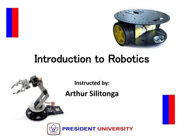
Introduction to Robotics. Instructed by: Arthur Silitonga. Outline. Course Information Course Overview & Objectives Course Materials Course Requirement/Evaluation/Grading (REG). I. Course Information. Instructor + Name : Arthur Silitonga + Address : Jl. Ki Hadjar Dewantara,

E N D
Introduction to Robotics Instructed by: Arthur Silitonga
Outline • Course Information • Course Overview & Objectives • Course Materials • Course Requirement/Evaluation/Grading (REG)
I. Course Information • Instructor + Name : Arthur Silitonga + Address : Jl. Ki Hadjar Dewantara, President University, Cikarang, Bekasi + Email Address : arthur@president.ac.id + Office Hours : Tuesday, 17.00 – 18.00 • Course‘s Meeting Time & Location + Meeting Time : Tuesday -> 10.30 – 13.00 (Lec) : Friday -> 07.30 – 10.00 (Lab) + Location : Room B, President University, Cikarang Baru, Bekasi
II. Course Overview & Objectives • Lecture sessions are tightly focused on introducing basic concepts of robotics from perspectives of mainly mechanics, control theory, and computer science. • Experiments at the lab occupying LEGO Mindstrom Kit, Wheeled Robot, and Robotic Atm. • Students are expected to design and implementing a real wheeled robot “from the scratch“. Course Overview
Course Objectives The objectives of this course are students should be able to : • describe positions and orientations in 3-space mathematically, and explain the geometry of mechanical manipulators generally • acquire concept of kinematics to velocities and static forces, general thought of forces & moments required to cause a motion of a manipulator, and sub-topics related to motions & mechanical designs of a manipulator • recognize methods of controlling a manipulator, and simulate the methods during lab works concerning to concepts of Wheeled Robot and Robotic Arm • design a wheeled robot “from the scratch“ based on knowledge of mechatronics To accomplish the objectives students will : • have homework assignments and participate in quizzes • implement calculations of 3-space positions & orientations using LEGO Mindstrom kit • design a wheeled robot considerating to theoretical and practical aspects • implement software aspects of a robotic arm • should take the mid-term exam, and the final exam
IV. Course Requirement/Evaluation/Grading • Requirements : - physics 1(mechanics) - linear algebra (matrix and vector) • Evaluation for the final grade will be based on : - Mid-Term Exam : 30 % - Final Exam : 30 % - Lab Experiments or Assignments : 20 % - Course Project : 20% Every two weeks, a quiz will be given as a preparation of several lab experiments
Mid-Term Exam consists of Lectures given in between the Week 1 and the Week 6. • Final Exam covers whole subjects or materials given duringthe classes. • Grading Policy Final grades may be adjusted; however, you are guaranteed the following: If your final score is 85 - 100, your grade will be A. If your final score is 70 - 84, your grade will be B. If your final score is 60 - 69, your grade will be C. If your final score is 55 - 59, your grade will beD. If your final score is < 55, your grade will be E.
REFERENCES • [Cra05]Craig, John., Introduction to Robotics : Mechanics and Control(Third Edition). Pearson Education, Inc.: New Jersey, USA. 2012. • [Sie04] Siegwart, Roland. & Nourbakhsh, Illah., Introduction to Autonomous Mobile Robots. The MIT Press : Cambridge, USA. 2004. • [Sic08]Siciliano, Bruno. & Khatib, Oussama., Handbook of Robotics. Springer-Verlag: Wuerzburg, Germany. 2008. • [Do08]Dorf, Richard. & Bishop, Robert., Modern Control Systems (Eleventh Edition). Pearson Education, Inc: Singapore, Singapore. 2008.
Introduction • Kinematics : science of motion that treats the subject without regard to the forces that cause it. position velocity acceleration all higher order derivatives of the position variables
Kinematics of manipulators refers to all the geometrical and time-based properties of the motion. • In this chapter, we consider position and orientation of the manipulator linkages in static situations.
The central topic of this chapter is a method to compute the position and orientation of the manipulator's end-effector relative to the base of the manipulator as a function of the joint variables.
Link Description • A manipulator may be thought of as a set of bodies connected in a chain by joints. • These bodies are called links. • Joints form a connection between a neighboring pair of links.
The term lower pair is used to describe the connection between a pair of bodies when the relative motion is characterized by two surfaces sliding over one another. Fig.10.1: The six possible lower-pair joints
A link is considered only as a rigid body that defines the relationship between two neighboring joint axes of a manipulator. • Joint axis i is defined by a line in space, or a vector direction, about which link i rotates relative to link i - 1.
Fig. 10.2: The kinematic function of a link is to maintain a fixed relationship between the two joint axes it supports.
Link Length : axis i and axis i – 1 (perpendicular) • Link twist : angle located on a plane whose normal is perpendicular line, and created by based on the difference of two axes
Link-Connector Description • In the investigation of kinematics, we need only worry about two quantities, which will completely specify the way in which links are connected together. Fig. 10.4: The link offset, d, and the joint angle, θ, are two parameters that may be used to describe the nature of the connection between neighboring links.
Intermediate links in the chain • Link offset : the distance along this common axis from one link to the next. • Joint angle, θi : the amount of rotation about this common axis between one link and its neighbor. • Figure 10.4 shows the interconnection of link i-1 and link i. Recall that at ai-1 is the mutual perpendicular between the two axes of link i — 1. Likewise, ai is the mutual perpendicular defined for link i. The first parameter of interconnection is the link offset, di, which is the signed distance measured along the axis of joint i from the point where ai-1 intersects the axis to the point where ai intersects the axis.
The link offset di is variable if joint i is prismatic. • The second parameter of interconnection is the angle made between an extension of ai-1 and ai measured about the axis of joint i. • This angle is named and is variable for a revolute joint.
First and last links in the chain • Link length ai, and link twist, αidepend on joint axes i and i + 1. • Hence, a1 through an-1 and α1through αn-1are defined as was discussed in this section. • At the ends of the chain, it will be our convention to assign zero to these quantities. That is, a0 = an = 0.0 and α0= αn = 0.0.
Link offset, and joint angle, are well defined for joints 2 through n — 1. • If joint 1 is revolute, the zero position for may be chosen arbitrarily, d1 = 0.0 will be our convention. • Similarly, if joint 1 is prismatic, the zero position of d1 may be chosen arbitrarily; d1= 0.0 will be our convention. Exactly the same statements apply to joint n.
Link parameters • A robot can be described kinematically by giving the values of four quantities for each link. Two describe the link itself, and two describe the link‘s connection to a neighboring link. • In the usual case of a revolute joint, θiis called the joint variable, and the other three quantities would be fixed link parameters. • For prismatic joints, d1 is the joint variable, and the other three quantities are fixed link parameters. The definition of mechanisms by means of these quantities is a convention usually called the Denavit—Hartenberg notation.
For a six-jointed robot, 18 numbers would be required to describe the fixed portion of its kinematics completely. • In the case of a six-jointed robot with all revolute joints, the 18 numbers are in the form of six sets of (αi, αi, di).
Convention For Affixing Frames To Links • In order to describe the location of each link relative to its neighbors, we define a frame attached to each link. • The link frames are named by number according to the link to which they are attached. That is, frame {i} is attached rigidly to link i.
Intermediate links in the chain • The convention we will use to locate frames on the links is as follows: The -axis of frame {i}, called , is coincident with the joint axis i. The origin of frame {i} is located where the ai perpendicular intersects the joint i axis. points along a1 in the direction from joint ito joint i + 1. • In the case of a1 = 0, is normal to the plane of and We define αi as being measured in the right-hand sense about and so we see that the freedom of choosing the sign of αiin this case corresponds to two choices for the direction of . is formed by the right-hand rule to complete the ith frame.
a c b
We attach a frame to the base of the robot, or link 0, called frame {0}. This frame does not move; for the problem of arm kinematics, it can be considered the reference frame. We may describe the position of all other link frames in terms of this frame. • Frame {0} is arbitrary, so it always simplifies matters to choose along axis 1 and to locate frame {0} so that it coincides with frame {1} when joint variable 1 is zero. • Using this convention, we will always have a0 = 0.0, α0 = 0.0. Additionally, this ensures that d1 = 0.0 if joint 1 is revolute, or θ1 = 0.0 if joint 1 is prismatic. First and last links in the chain
Fig. 10.5: Link frames are attached so that frame {i} is attached rigidly to link i.
Summary of the link parameters in terms of the link frames • If the link frames have been attached to the links according to our convention, the following definitions of the link parameters are valid: • We usually choose ai > 0, because it corresponds to a distance; however, and are signed quantities.
Summary of the link parameters in terms of the link frames • The following is a summary of the procedure to follow when faced with a new mechanism, in order to properly attach the link frames: 1. Identify the joint axes and imagine (or draw) infinite lines along them. steps 2 through 5 below, consider two of these neighboring lines (at axes i and i + 1). 2. Identify the common perpendicular between them, or point of intersection. At the point of intersection, or at the point where the common perpendicular meets the ith axis, assign the link-frame origin. 3. Assign the axis pointing along the ith joint axis. 4. Assign the axis pointing along the common perpendicular, or, if the axes intersect, assign to be normal to the plane containing the two axes.
5. Assign the axis to complete a right-hand coordinate system. 6. Assign {0} to match {1} when the first joint variable is zero. For {N}, choose an origin location and direction freely, but generally so as to cause as many linkage parameters as possible to become zero.
MANIPULATOR KINEMATICS • We derive the general form of the transformation that relates the frames attached to neighboring links. • We then concatenate these individual transformations to solve for the position and orientation of link n relative to link 0.
We wish to construct the transform that defines frame {i } relative to the frame {i — 1}. • In general, this transformation will be a function of the four link parameters. For any given robot, this transformation will be a function of only one variable, the other three parameters being fixed by mechanical design. Derivation of link transformations
Each of these four transformations will be a function of one link parameter oniy and will be simple enough that we can write down its form by inspection. • We begin by defining three intermediate frames for each link—{P}, {Q}, and {R}. • Figure 10.15 shows the same pair of joints as before with frames {P}, {Q}, and {R} defined. • Note that only the and axes are shown for each frame, to make the drawing clearer. Frame {R} differs from frame {i - 1} only by a rotation of
Frame (Q} differs from {R} by a translation ai-1. Frame {P} differs from {Q} by a rotation and frame {i} differs from {P} by a translation di.
Fig. 10.15: Location of intermediate frames {P}, {Q}, and {R}. Frame (Q} differs from {R} by a translation ai-1. Frame {P} differs from {Q} by a rotation and frame {i} differs from {P} by a translation di. If we wish to write the transformation that transforms vectors defined in {i} to their description in {i – 1} we may write
Considering each of these transformations, we see that the last mentioned equation may be written where the notation ScrewQ(r, θ) stands for the combination of a translation along an axis by a distance r and a rotation about the same axis by an angle
Once the link frames have been defined and the corresponding link parameters found, developing the kinematic equations is straightforward. • From the values of the link parameters, the individual link-transformation matrices can be computed. • Then, the link transformations can be multiplied together to find the single transformation that relates frame [N} to frame {0}: • This transformation, , will be a function of all ii joint variables. If the robot's joint-position sensors are queried, the Cartesian position and orientation of the last link can be computed by Concatenating Link Transformations
ACTUATOR SPACE, JOINT SPACE, AND CARTESIAN SPACE • The position of all the links of a manipulator of n degrees of freedom can be specified with a set of n joint variables. • This set of variables is often referred to as the a x 1 joint vector. • The space of all such joint vectors is referred to as joint space. • We have been concerned with computing the Cartesian space description from knowledge of the joint-space description. • We use the term Cartesian space when position is measured along orthogonal axes and orientation is measured according to any of the conventions. • Sometimes, the terms task-oriented space and operational space are used for what we will call Cartesianspace.
Fig. 10.16: Mappings between kinematic descriptions • There are three representations of a manipulator's position and orientation: • descriptions in actuator space, in joint space, and in Cartesian space • The ways in which actuators might be connected to move a joint are quite varied; • they might be catalogued, but we wifi not do so here. For each robot we • design or seek to analyze, the correspondence between actuator positions and • joint positions must be solved
EXAMPLES: KINEMATICS OF TWO INDUSTRIAL ROBOTS • Current industrial robots are available in many different kinematic configurations. • In this section, we work out the kinematics of two typical industrial robots. First we consider the Unimation PUMA 560, a rotary-joint manipulator with six degrees of freedom. • Kinematic equations as functions of the joint angles will be solved. • For this example, we will skip the additional problem of the relationship between actuator space and joint space. • Second, we consider the Yasukawa Motoman L-3, a robot with five degrees of freedom and rotary joints. This example is done in detail, including the actuator-to-joint transformations.