Level Set Methods
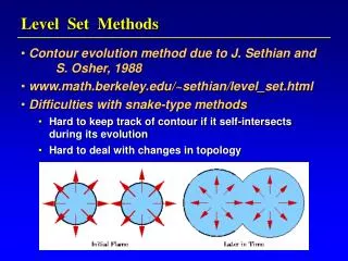
Level Set Methods. Contour evolution method due to J. Sethian and S. Osher, 1988 www.math.berkeley.edu/~sethian/level_set.html Difficulties with snake-type methods Hard to keep track of contour if it self-intersects during its evolution Hard to deal with changes in topology .

Level Set Methods
E N D
Presentation Transcript
Level Set Methods • Contour evolution method due to J. Sethian and S. Osher, 1988 • www.math.berkeley.edu/~sethian/level_set.html • Difficulties with snake-type methods • Hard to keep track of contour if it self-intersects during its evolution • Hard to deal with changes in topology
The level set approach: • Define problem in 1 higher dimension • Define level set function z = (x,y,t = 0) where the (x,y) plane contains the contour, and z = signed Euclidean distance transform value (negative means inside closed contour, positive means outside contour)
How to Move the Contour? • Move the level set function, (x,y,t), so that it rises, falls, expands, etc. • Contour = cross section at z = 0, i.e., {(x,y) | (x,y,t) = 0}
Level Set Surface • The zero level set (in blue) at one point in time as a slice of the level set surface (in red)
Level Set Surface • Later in time the level set surface (red) has moved and the new zero level set (blue) defines the new contour
How to Move the Level Set Surface? • Define a velocity field, F, that specifies how contour points move in time • Based on application-specific physics such as time, position, normal, curvature, image gradient magnitude • Build an initial value for the level set function, (x,y,t=0), based on the initial contour position • Adjust over time; contour at time t defined by (x(t), y(t), t) = 0 Hamilton-Jacobi equation
Level Set Formulation • Constraint: level set value of a point on the contour with motion x(t) must always be 0 (x(t), t) = 0 • By the chain rule t+ (x(t), t) · x(t) = 0 • Since F supplies the speed in the outward normal direction x(t) · n = F, where n = / || • Hence evolution equation for is t + F|| = 0
Example: Shape Simplification • F = 1 – 0.1 where is the curvature at each contour point
Example: Segmentation • Digital Subtraction Angiogram • F based on image gradient and contour curvature
Example (cont.) • Initial contour specified manually
Fast Marching Method • J. Sethian, 1996 • Special case that assumes the velocity field, F, never changes sign. That is, contour is either always expanding (F>0) or always shrinking (F<0) • Convert problem to a stationary formulation on a discrete grid where the contour is guaranteed to cross each grid point at most once
Fast Marching Method • Compute T(x,y) = time at which the contour crosses grid point (x,y) • At any height, t, the surface gives the set of points reached at time t
Fast Marching Algorithm • Compute T using the fact that • Distance = rate×time • In 1D: 1 = F×dT/dx • In 2D: 1 = F× | T | • Contour at time t = {(x,y) | T(x,y) = t}
Fast Marching Algorithm • Construct the arrival time surface T(x,y) incrementally: • Build the initial contour • Incrementally add on to the existing surface the part that corresponds to the contour moving with speed F (in other words, repeatedly pick a point on the fringe with minimum T value) • Iterate until F goes to 0 • Builds level set surface by “scaffolding” the surface patches farther and farther away from the initial contour
Fast Marching Update “downwind” (i.e., unvisited neighbors) Compute new possible values
Fast Marching Expand point on the fringe with minimum value Update neighbors “downwind”
Fast Marching Expand point on the fringe with minimum value Update neighbors “downwind”
Fast Marching + Level Set for Shape Recovery • First use the Fast Marching algorithm to obtain “rough” contour • Then use the Level Set algorithm to fine tune, using a few iterations, the results from Fast Marching
Results: Segmentation using Fast Marching No level set tuning
Results: Vein Segmentation No level set tuning With level set tuning
Results: Vein Segmentation (continued) Original Fast Marching + Level Set onlyLevel Set Tuning
Results: Segmentation using Fast Marching No level set tuning
Results: Brain Image Segmentation # of iterations = 9000 # of iterations = 12000 Fast marching only, no level set tuning
Results: Brain Segmentation (continued) Without level set tuning With level set tuning
Results: Segmentation using Fast Marching No level set tuning