Download

1 / 36
390 likes | 442 Vues
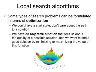
Dive into local search algorithms, effective for large problems but not always optimal. Learn to keep and improve states iteratively, seeking complete configurations. Explore examples like n-Queens and VLSI layout. Understand algorithm design considerations and random restart techniques to enhance search outcomes.

E N D
Local search algorithms CS271P, Winter Quarter, 2019 Introduction to Artificial Intelligence Prof. Richard Lathrop Read Beforehand: R&N 4.1-4.2, 4.6 Optional: R&N 4.3-4.5
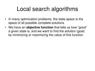
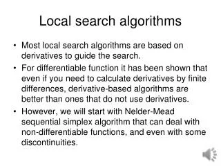
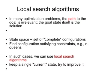
Local search algorithms • In many optimization problems, the path to the goal is irrelevant; the goal state itself is the solution • Local search: widely used for very bigproblems • Returns good but not optimalsolutions • Usually very slow, but can yield good solutions if you wait • State space = set of "complete" configurations • Find a complete configuration satisfying constraints • Examples: n-Queens, VLSI layout, airline flight schedules • Local search algorithms • Keep a single "current" state, or small set of states • Iteratively try to improve it / them • Very memory efficient • keeps only one or a few states • You control how much memory you use
Basic idea of local search (many variations) // initialize to something, usually a random initial state // alternatively, might pass in a human-generated initial state best_found ← current_state ← RandomState() // now do local search loop do if (tired of doing it) then returnbest_found else current_state←MakeNeighbor( current_state ) if ( Cost(current_state) < Cost(best_found) ) then // keep best result found so far best_found ← current_state You, as algorithm designer, write the functions named in red. Typically, “tired of doing it” means that some resource limit is exceeded, e.g., number of iterations, wall clock time, CPU time, etc. It may also mean that result improvements are small and infrequent, e.g., less than 0.1% result improvement in the last week of run time.
Example: n-queens • Goal: Put n queens on an n × n board with no two queens on the same row, column, or diagonal • Neighbor: move one queen to another row • Search: go from one neighbor to the next…
Algorithm design considerations • How do you represent your problem? • What is a “complete state”? • What is your objective function? • How do you measure cost or value of a state? • Stand on your head: cost = −value, value = −cost • What is a “neighbor” of a state? • Or, what is a “step” from one state to another? • How can you compute a neighbor or a step? • Are there any constraints you can exploit?
Random restart wrapper • We’ll use stochastic local search methods • Return different solution for each trial & initial state • Almost every trial hits difficulties (see sequel) • Most trials will not yield a good result (sad!) • Using many random restarts improves your chances • Many “shots at goal” may finally get a good one • Restart a random initial state, many times • Report the best result found across many trials
Random restart wrapper best_found←RandomState()// initialize to something // now do repeated local search loop do if(tired of doing it) then returnbest_found else result←LocalSearch( RandomState() ) if ( Cost(result) < Cost(best_found) ) // keep best result found so far thenbest_found←result You, as algorithm designer, write the functions named in red. Typically, “tired of doing it” means that some resource limit has been exceeded, e.g., number of iterations, wall clock time, CPU time, etc. It may also mean that result improvements are small and infrequent, e.g., less than 0.1% result improvement in the last week of run time.
Tabu search wrapper • Add recently visited states to a tabu-list • Temporarily excluded from being visited again • Forces solver away from explored regions • Less likely to get stuck in local minima (hope, in principle) • Implemented as a hash table + FIFO queue • Unit time cost per step; constant memory cost • You control how much memory is used • RandomRestart( TabuSearch ( LocalSearch() ) )
Tabu search wrapper(inside random restart! ) New State Oldest State FIFO QUEUE HASH TABLE best_found ← current_state ← RandomState() // initialize loop do // now do local search if (tired of doing it) then returnbest_foundelse neighbor←MakeNeighbor( current_state ) if ( neighbor is in hash_table ) then discard neighbor else push neighbor onto fifo, pop oldest_state remove oldest_state from hash_table, insert neighbor current_state ← neighbor; if ( Cost(current_state ) < Cost(best_found) ) then best_found ← current_state State Present?
Local search algorithms • Hill-climbing search • Gradient descent in continuous state spaces • Can use, e.g., Newton’s method to find roots • Simulated annealing search • Local beam search • Genetic algorithms • Linear Programming (for specialized problems)
Local Search Difficulties These difficulties apply to ALL local search algorithms, and become MUCH more difficult as the search space increases to high dimensionality. • Problems: depending on state, can get stuck in local maxima • Many other problems also endanger your success!!
Local Search Difficulties These difficulties apply to ALL local search algorithms, and become MUCH more difficult as the search space increases to high dimensionality. • Ridge problem: Every neighbor appears to be downhill • But the search space has an uphill!! (worse in high dimensions) Ridge: Fold a piece of paper and hold it tilted up at an unfavorable angle to every possible search space step. Every step leads downhill; but the ridge leads uphill.
Hill-climbing search You must shift effortlessly between maximizing value and minimizing cost “…like trying to find the top of Mount Everest in a thick fog while suffering from amnesia” Equivalently: “…a lowest-cost successor…” Equivalently: “if COST[neighbor] COST[current] then …”
Example: Hill-climbing, 8-queens h = # of pairs of queens that are attacking each other, either directly or indirectly (cost) h=17 for this state Each number indicates h if we move a queen in its column to that square 12 (boxed) = best h among all neighors; select one randomly
Example: Hill-climbing, 8-queens • A local minimum with h=1 • All one-step neighbors have higher h values • What can you do to get out of this local minimum?
Gradient descent • Hill-climbing in continuous state spaces • Denote “state” as θ, a vector of parameters • Denote cost as J(θ) • How to change θto improve J(θ)? • Choose a direction in which J(θ) is decreasing • Derivative • Positive => increasing cost • Negative => decreasing cost The curly D means to take a derivative while holding all other variables constant. You are not responsible for multivariate calculus, but gradient descent is a very important method, so it is presented.
Gradient descent Hill-climbing in continuous spaces • Gradient vector • Gradient = direction of steepest ascent • Negative gradient = steepest descent (c) Alexander Ihler
Gradient descent Hill-climbing in continuous spaces Gradient = the most direct direction up-hill in the objective (cost) function, so its negative minimizes the cost function. * Assume we have some cost-function: and we want minimize over continuous variables x1,x2,..,xn 1. Compute the gradient : 2.Take a small step downhill in the direction of the gradient: 3. Check if 4. If true then accept move, if not “reject”. 5. Repeat. (or, Armijo rule, etc.) (decrease step size, etc.)
Gradient descent Hill-climbing in continuous spaces • How do I determine the gradient? • Derive formula using multivariate calculus. • Ask a mathematician or a domain expert. • Do a literature search. • Variations of gradient descent can improve performance for this or that special case. • See Numerical Recipes in C (and in other languages) by Press, Teukolsky, Vetterling, and Flannery. • Simulated Annealing, Linear Programming too • Works well in smooth spaces; poorly in rough.
Newton’s method • Want to find the roots of f(x) • “Root”: value of x for which f(x)=0 • Initialize to some point xn • Compute the tangent at xn & compute xn+1 = where it crosses x-axis
Newton’s method • Want to find the roots of f(x) • “Root”: value of x for which f(x)=0 • Initialize to some point xn • Compute the tangent at xn & compute xn+1 = where it crosses x-axis • Repeat for xn+1 • Does not always converge; sometimes unstable • If converges, usually very fast • Works well for smooth, non-pathological functions; accurate linearization • Works poorly for wiggly, ill-behaved functions; tangent is a poor guide to root
Simulated annealing (Physics!) • Idea: escape local maxima by allowing some "bad" moves but gradually decrease their frequency Improvement: Track the BestResultFoundSoFar. Here, this slide follows Fig. 4.5 of the textbook, which is simplified.
Typical annealing schedule • Usually use a decaying exponential • Axis values scaled to fit problem characteristics Temperature
Probability( accept worse successor ) • Decreases as temperature T decreases • Increases as |Δ E| decreases • Sometimes, step size also decreases with T (accept very bad moves early on; later, mainly accept “not very much worse”) Temperature
Goal: “ratchet up” a bumpy slope(see HW #2, prob. #5; here T = 1; cartoon is NOT to scale) G Value=51 E Value=48 Value C Value=45 A Value=42 F Value=47 D Value=44 B Value=41 Arbitrary (Fictitious) Search Space Coordinate Your “random restart wrapper” starts here. You want to get here. HOW?? This is an illustrative cartoon…
Goal: “ratchet up” a jagged slope E Value=48 E(ED)=-4 E(EF)=-1 P(ED) .018 P(EF).37 C Value=45 E(CB)=-4 E(CD)=-1 P(CB) .018 P(CD).37 A Value=42 E(AB)=-1 P(AB) .37 G Value=51 E(GF)=-4 P(GF) .018 F Value=47 E(FE)=1 E(FG)=4 P(FE)=1 P(FG)=1 D Value=44 E(DC)=1 E(DE)=4 P(DC)=1 P(DE)=1 B Value=41 E(BA)=1 E(BC)=4 P(BA)=1 P(BC)=1 Your “random restart wrapper” starts here. From A you will accept a move to B with P(AB) .37. From B you are equally likely to go to A or to C. From C you are 20X more likely to go to D than to B. From D you are equally likely to go to C or to E. From E you are 20X more likely to go to F than to D. From F you are equally likely to go to E or to G. Remember best point you ever found (G or neighbor?). This is an illustrative cartoon…
Properties of simulated annealing • One can prove: • If T decreases slowly enough, then simulated annealing search will find a global optimum with probability approaching 1 • Unfortunately this can take a VERY VERY long time • Note: in any finite search space, random guessing also will find a global optimum with probability approaching 1 • So, ultimately this is a very weak claim • Often works very well in practice • But usually VERY VERY slow • Widely used in VLSI layout, airline scheduling, etc.
Local beam search • Keep track of k states rather than just one • Start with k randomly generated states • At each iteration, all the successors of all k states are generated • If any one is a goal state, stop; else select the k best successors from the complete list and repeat. • Concentrates search effort in areas believed to be fruitful • May lose diversity as search progresses, resulting in wasted effort
Local beam search … … Create k random initial states Select the k best children a1 b1 a2 b2 k1 k2 … … Generate their children Repeat indefinitely… Is it better than simply running k searches? Maybe…??
Genetic algorithms (Darwin!!) • A state = a string over a finite alphabet (an individual) • A successor state is generated by combining two parent states • Start with k randomly generated states (a population) • Fitness function (= our heuristic objective function). • Higher fitness values for better states. • Select individuals for next generation based on fitness • P(individual in next gen.) = individual fitness/total population fitness • Crossover fit parents to yield next generation (offspring) • Mutate the offspring randomly with some low probability
Example: N-Queens Each “individual” is a vector of each queen’s row
Genetic algorithms • Fitness function (value): number of non-attacking pairs of queens (min = 0, max = 8 × 7/2 = 28) • 24/(24+23+20+11) = 31% • 23/(24+23+20+11) = 29%; etc.
fitness = #non-attacking queens probability of being in next generation = fitness/(_i fitness_i) How to convert a fitness value into a probability of being in the next generation. • Fitness function: #non-attacking queen pairs • min = 0, max = 8 × 7/2 = 28 • i fitness_i = 24+23+20+11 = 78 • P(pick child_1 for next gen.) = fitness_1/(_i fitness_i) = 24/78 = 31% • P(pick child_2 for next gen.) = fitness_2/(_i fitness_i) = 23/78 = 29%; etc
Linear Programming • Maximize: z = c1 x1 + c2 x2 +…+ cnxn • Primary constraints: x10, x20, …, xn0 • Arbitrary additional linear constraints: ai1 x1 + ai2 x2 + … + ainxn ai, (ai 0) aj1 x1 + aj2 x2 + … + ajnxn aj 0 bk1 x1 + bk2 x2 + … + bknxn= bk 0 • Restricted class of linear problems. • Efficient for very large problems(!!) in this class.
Linear ProgrammingEfficient Optimal SolutionFor a Restricted Class of Problems • Very efficient “off-the-shelf” solvers are available for LPs. • They quickly solve large problems with thousands of variables.
Summary • Local search maintains a complete solution • Maintains a complete solution, seeks consistent (or at least good) • vs: Path search maintains a consistent solution; seeks complete • Goal of both: consistent & complete solution • Types: • hill climbing, gradient ascent • simulated annealing, other Monte Carlo methods • Population methods: beam search; genetic / evolutionary algorithms • Wrappers: random restart; tabu search • Local search often works well on very large problems • Abandons optimality • Always has some answer available (best found so far) • Often requires a very long time to achieve a good result