4 Greedy Algorithms
4 Greedy Algorithms. Interval Scheduling Scheduling Jobs Shortest Path Algorithms Minimum Spanning Tree Algorithms Clustering. 4.1 Interval Scheduling. Interval Scheduling. Interval scheduling. Job j starts at s j and finishes at f j . Two jobs compatible if they don't overlap.

4 Greedy Algorithms
E N D
Presentation Transcript
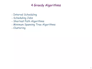
4 Greedy Algorithms • Interval Scheduling • Scheduling Jobs • Shortest Path Algorithms • Minimum Spanning Tree Algorithms • Clustering
Interval Scheduling • Interval scheduling. • Job j starts at sj and finishes at fj. • Two jobs compatible if they don't overlap. • Goal: find maximum subset of mutually compatible jobs. a b c d e f g h Time 0 1 2 3 4 5 6 7 8 9 10 11
Interval Scheduling: Greedy Algorithms • Greedy template. Consider jobs in some order. Take each job provided it's compatible with the ones already taken. • [Earliest start time] Consider jobs in ascending order of start time sj. • [Earliest finish time] Consider jobs in ascending order of finish time fj. • [Shortest interval] Consider jobs in ascending order of interval length fj - sj. • [Fewest conflicts] For each job, count the number of conflicting jobs cj. Schedule in ascending order of conflicts cj.
Interval Scheduling: Greedy Algorithms • Greedy template. Consider jobs in some order. Take each job provided it's compatible with the ones already taken. breaks earliest start time breaks shortest interval breaks fewest conflicts
Interval Scheduling: Greedy Algorithm • Greedy algorithm. Consider jobs in increasing order of finish time. Take each job provided it's compatible with the ones already taken. • Implementation. O(n log n). • Remember job j* that was added last to A. • Job j is compatible with A if sj fj*. Sort jobs by finish times so that f1 f2 ... fn. A for j = 1 to n { if (job j compatible with A) A A {j} } return A jobs selected
Interval Scheduling: Analysis • Theorem. Greedy algorithm is optimal. • Pf. (by contradiction) • Assume greedy is not optimal, and let's see what happens. • Let i1, i2, ... ik denote set of jobs selected by greedy. • Let j1, j2, ... jm denote set of jobs in the optimal solution withi1 = j1, i2 = j2, ..., ir = jr for the largest possible value of r. job ir+1 finishes before jr+1 Greedy: i1 i1 ir ir+1 OPT: j1 j2 jr jr+1 . . . why not replace job jr+1with job ir+1?
Interval Scheduling: Analysis • Theorem. Greedy algorithm is optimal. • Pf. (by contradiction) • Assume greedy is not optimal, and let's see what happens. • Let i1, i2, ... ik denote set of jobs selected by greedy. • Let j1, j2, ... jm denote set of jobs in the optimal solution withi1 = j1, i2 = j2, ..., ir = jr for the largest possible value of r. job ir+1 finishes before jr+1 Greedy: i1 i1 ir ir+1 OPT: j1 j2 jr ir+1 . . . solution still feasible and optimal, but contradicts maximality of r.
Interval Scheduling : Example B C A E D F G H Time 0 1 2 3 4 5 6 7 8 9 10 11 0 1 2 3 4 5 6 7 8 9 10 11
Interval Scheduling B C A E D F G H Time 0 1 2 3 4 5 6 7 8 9 10 11 B 0 1 2 3 4 5 6 7 8 9 10 11
Interval Scheduling B C A E D F G H Time 0 1 2 3 4 5 6 7 8 9 10 11 B C 0 1 2 3 4 5 6 7 8 9 10 11
Interval Scheduling B C A E D F G H Time 0 1 2 3 4 5 6 7 8 9 10 11 A B 0 1 2 3 4 5 6 7 8 9 10 11
Interval Scheduling B C A E D F G H Time 0 1 2 3 4 5 6 7 8 9 10 11 B E 0 1 2 3 4 5 6 7 8 9 10 11
Interval Scheduling B C A E D F G H Time 0 1 2 3 4 5 6 7 8 9 10 11 B D E 0 1 2 3 4 5 6 7 8 9 10 11
Interval Scheduling B C A E D F G H Time 0 1 2 3 4 5 6 7 8 9 10 11 B E F 0 1 2 3 4 5 6 7 8 9 10 11
Interval Scheduling B C A E D F G H Time 0 1 2 3 4 5 6 7 8 9 10 11 B E G 0 1 2 3 4 5 6 7 8 9 10 11
Interval Scheduling B C A E D F G H Time 0 1 2 3 4 5 6 7 8 9 10 11 B E H 0 1 2 3 4 5 6 7 8 9 10 11
Interval Partitioning • Interval partitioning. • Lecture j starts at sj and finishes at fj. • Goal: find minimum number of classrooms to schedule all lectures so that no two occur at the same time in the same room. • Ex: This schedule uses 4 classrooms to schedule 10 lectures. e j g c d b h a f i 3 3:30 4 4:30 9 9:30 10 10:30 11 11:30 12 12:30 1 1:30 2 2:30 Time
Interval Partitioning • Interval partitioning. • Lecture j starts at sj and finishes at fj. • Goal: find minimum number of classrooms to schedule all lectures so that no two occur at the same time in the same room. • Ex: This schedule uses only 3. f c d j i b g a h e 3 3:30 4 4:30 9 9:30 10 10:30 11 11:30 12 12:30 1 1:30 2 2:30 Time
Interval Partitioning: Lower Bound on Optimal Solution • Def. The depth of a set of open intervals is the maximum number that contain any given time. • Key observation. Number of classrooms needed depth. • Ex: Depth of schedule below = 3 schedule below is optimal. • Q. Does there always exist a schedule equal to depth of intervals? a, b, c all contain 9:30 f c d j i b g a h e 3 3:30 4 4:30 9 9:30 10 10:30 11 11:30 12 12:30 1 1:30 2 2:30 Time
Interval Partitioning: Greedy Algorithm • Greedy algorithm. Consider lectures in increasing order of start time: assign lecture to any compatible classroom. • Implementation. O(n log n). • For each classroom k, maintain the finish time of the last job added. • Keep the classrooms in a priority queue. Sort intervals by starting time so that s1 s2 ... sn. d 0 for j = 1 to n { if (lecture j is compatible with some classroom k) schedule lecture j in classroom k else allocate a new classroom d + 1 schedule lecture j in classroom d + 1 d d + 1 } number of allocated classrooms
Interval Partitioning: Greedy Analysis • Observation. Greedy algorithm never schedules two incompatible lectures in the same classroom. • Theorem. Greedy algorithm is optimal. • Pf. • Let d = number of classrooms that the greedy algorithm allocates. • Classroom d is opened because we needed to schedule a job, say j, that is incompatible with all d-1 other classrooms. • Since we sorted by start time, all these incompatibilities are caused by lectures that start no later than sj. • Thus, we have d lectures overlapping at time sj + . • Key observation all schedules use d classrooms. ▪
1 2 3 4 5 6 tj 3 2 1 4 3 2 dj 6 8 9 9 14 15 Scheduling to Minimizing Lateness • Minimizing lateness problem. • Single resource processes one job at a time. • Job j requires tj units of processing time and is due at time dj. • If j starts at time sj, it finishes at time fj = sj + tj. • Lateness: j = max { 0, fj - dj }. • Goal: schedule all jobs to minimize maximumlateness L = max j. • Ex: lateness = 2 lateness = 0 max lateness = 6 d3 = 9 d2 = 8 d6 = 15 d1 = 6 d5 = 14 d4 = 9 12 13 14 15 0 1 2 3 4 5 6 7 8 9 10 11
Minimizing Lateness: Greedy Algorithms • Greedy template. Consider jobs in some order. • [Shortest processing time first] Consider jobs in ascending order of processing time tj. • [Earliest deadline first] Consider jobs in ascending order of deadline dj. • [Smallest slack] Consider jobs in ascending order of slack dj - tj.
1 1 2 2 1 1 10 10 2 100 10 10 Minimizing Lateness: Greedy Algorithms • Greedy template. Consider jobs in some order. • [Shortest processing time first] Consider jobs in ascending order of processing time tj. • [Smallest slack] Consider jobs in ascending order of slack dj - tj. tj counterexample dj tj counterexample dj
d1 = 6 d2 = 8 d3 = 9 d4 = 9 d5 = 14 d6 = 15 Minimizing Lateness: Greedy Algorithm • Greedy algorithm. Earliest deadline first. Sort n jobs by deadline so that d1 d2 … dn t 0 for j = 1 to n Assign job j to interval [t, t + tj] sj t, fj t + tj t t + tj output intervals [sj, fj] max lateness = 1 12 13 14 15 0 1 2 3 4 5 6 7 8 9 10 11
Minimizing Lateness: No Idle Time • Observation. There exists an optimal schedule with noidle time. • Observation. The greedy schedule has no idle time. d = 4 d = 6 d = 12 0 1 2 3 4 5 6 7 8 9 10 11 d = 4 d = 6 d = 12 0 1 2 3 4 5 6 7 8 9 10 11
Minimizing Lateness: Inversions • Def. An inversion in schedule S is a pair of jobs i and j such that:i < j but j scheduled before i. • Observation. Greedy schedule has no inversions. • Observation. If a schedule (with no idle time) has an inversion, it has one with a pair of inverted jobs scheduled consecutively. inversion before swap j i
Minimizing Lateness: Inversions • Def. An inversion in schedule S is a pair of jobs i and j such that:i < j but j scheduled before i. • Claim. Swapping two adjacent, inverted jobs reduces the number of inversions by one and does not increase the max lateness. • Pf. Let be the lateness before the swap, and let ' be it afterwards. • 'k = k for all k i, j • 'ii • If job j is late: inversion fi before swap j i after swap i j f'j
Minimizing Lateness: Analysis of Greedy Algorithm • Theorem. Greedy schedule S is optimal. • Pf. Define S* to be an optimal schedule that has the fewest number of inversions, and let's see what happens. • Can assume S* has no idle time. • If S* has no inversions, then S = S*. • If S* has an inversion, let i-j be an adjacent inversion. • swapping i and j does not increase the maximum lateness and strictly decreases the number of inversions • this contradicts definition of S* ▪
Greedy Analysis Strategies • Greedy algorithm stays ahead. Show that after each step of the greedy algorithm, its solution is at least as good as any other algorithm's. • Exchange argument. Gradually transform any solution to the one found by the greedy algorithm without hurting its quality. • Structural. Discover a simple "structural" bound asserting that every possible solution must have a certain value. Then show that your algorithm always achieves this bound.
Optimal Offline Caching • Caching. • Cache with capacity to store k items. • Sequence of m item requests d1, d2, …, dm. • Cache hit: item already in cache when requested. • Cache miss: item not already in cache when requested: must bring requested item into cache, and evict some existing item, if full. • Goal. Eviction schedule that minimizes number of cache misses. • Ex: k = 2, initial cache = ab, requests: a, b, c, b, c, a, a, b. • Optimal eviction schedule: 2 cache misses. a a b b a b c c b b c b c c b a a b a a b b a b cache requests
Optimal Offline Caching: Farthest-In-Future • Farthest-in-future. Evict item in the cache that is not requested until farthest in the future. • Theorem. [Bellady, 1960s]FF is optimal eviction schedule. • Pf. Algorithm and theorem are intuitive; proof is subtle. current cache: a b c d e f future queries: g a b c e d a b b a c d e a f a d e f g h ... eject this one cache miss
Reduced Eviction Schedules • Def. A reduced schedule is a schedule that only inserts an item into the cache in a step in which that item is requested. • Intuition. Can transform an unreduced schedule into a reduced one with no more cache misses. a a b c a a b c a a x c a a b c c a d c c a b c d a d b d a d c a a c b a a d c b a x b b a d b c a c b c a c b a a b c a a c b a a b c a a c b an unreduced schedule a reduced schedule
Reduced Eviction Schedules • Claim. Given any unreduced schedule S, can transform it into a reduced schedule S' with no more cache misses. • Pf. (by induction on number of unreduced items) • Suppose S brings d into the cache at time t, without a request. • Let c be the item S evicts when it brings d into the cache. • Case 1: d evicted at time t', before next request for d. • Case 2: d requested at time t' before d is evicted. ▪ doesn't enter cache at requested time S S' S S' c c c c t t t t d d t' t' t' t' e e d d evicted at time t',before next request d requested at time t' Case 1 Case 2
Farthest-In-Future: Analysis • Theorem. FF is optimal eviction algorithm. • Pf. (by induction on number or requests j) • Let S be reduced schedule that satisfies invariant through j requests. We produce S' that satisfies invariant after j+1 requests. • Consider (j+1)st request d = dj+1. • Since S and SFF have agreed up until now, they have the same cache contents before request j+1. • Case 1: (d is already in the cache). S' = S satisfies invariant. • Case 2: (d is not in the cache and S and SFF evict the same element).S' = S satisfies invariant. Invariant: There exists an optimal reduced schedule S that makes the same eviction schedule as SFF through the first j+1 requests.
Farthest-In-Future: Analysis • Pf. (continued) • Case 3: (d is not in the cache; SFF evicts e; S evicts f e). • begin construction of S' from S by evicting e instead of f • now S' agrees with SFF on first j+1 requests; we show that having element f in cache is no worse than having element e same e f same e f j S S' same e d same d f j+1 j S S'
Farthest-In-Future: Analysis • Let j' be the first time after j+1 that S and S' take a different action, and let g be item requested at time j'. • Case 3a: g = e. Can't happen with Farthest-In-Future since there must be a request for f before e. • Case 3b: g = f. Element f can't be in cache of S, so let e' be the element that S evicts. • if e' = e, S' accesses f from cache; now S and S' have same cache • if e' e, S' evicts e' and brings e into the cache; now S and S' have the same cache must involve e or f (or both) j' same e same f S S' Note: S' is no longer reduced, but can be transformed intoa reduced schedule that agrees with SFF through step j+1