Download
1 / 17
190 likes | 515 Vues
Quantum Mechanics Calculations. Noel M. O’Boyle. Apr 2010 Postgrad course on Comp Chem. Overview of QM methods. Molecular mechanics. Quantum mechanics (wavefunction). Quantum mechanics (electron density). Including correlation HF (“ab initio”) Semi-empirical. DFT. Speed/Accuracy.

E N D
Quantum Mechanics Calculations Noel M. O’Boyle Apr 2010 Postgrad course on Comp Chem
Overview of QM methods Molecular mechanics Quantum mechanics (wavefunction) Quantum mechanics (electron density) Including correlation HF (“ab initio”) Semi-empirical DFT Speed/Accuracy Forcefields
What can be calculated? • Molecular orbitals and their energies • Electron density • Molecular geometry • Relative energies of two molecules • NMR shifts • IR and Raman frequencies and normal modes • Electronic transitions (UV-Vis absorption spectrum), associated changes in electron density, optical rotation • Conductivity • Ionisation potential, electron affinity, heat of formation • Transition states, activation energy • Charge distribution • Interaction energy between two molecules • Solvation energy • pKa How accurately can it be calculated?...
References • Essentials of Computational Chemistry, Christopher Cramer • Introduction to Computational Chemistry, Frank Jensen • Molecular Modelling: Principles and Applications, Andrew Leach • Computational Organic Chemistry, Steven Bachrach(http://comporgchem.com/blog/) • (coming soon) Molecular Modelling Basics, Jan Jensen (http://molecularmodelingbasics.blogspot.com/) • Quantum Mechanics, Tim Clark, Section 7.4 in Cheminformatics– A Textbook, Ed. Gasteiger and Engel
The Wavefunction • The wavefunction completely describes the properties of a quantum mechanical (QM) system • Ψ(r), Psi • It has a value at every point in 3D space • By applying various operators to the wavefunction, we can calculate properties of the system • The Hamiltonian operator (Ĥ) gives the energy of the system • ĤΨ=EΨ (the Schrödinger equation) • ρ = |Ψ|2 • “electron density” or “square or the wavefunction” • A probability density (3D) • Integrate over a certain volume to find the probability of finding an electron in that volume • It follows that ∫|Ψ|2dr = N (number of electrons) Credit: OtherDrK (Flickr)
Solving the Schrodinger equation • Born-Oppenheimer approximation • Since electron motion is so rapid compared to nuclear motion, consider the nuclei as fixed • This allows us to simplify the Hamilitonian • Variational Principle • The true energy of a QM system (as given by the Hamilitonian operator) is always less than the energy found if the Hamilitonian is applied to an incorrect wavefunction • To find the true wavefunction, make a reasonable guess and then keep altering it to minimise the energy • Hartree-Fock (HF) theory • HF theory neglects electron correlation in multi-electron systems • Instead, we imagine each electron interacting with a static field of all of the other electrons • According to the variational principle, the lowest energy will can get with HF theory will always be greater than the true energy of the system • The difference is the correlation energy
Expressing a vector in terms of a basis (3.5, 1.5) v j i v = 3.5i + 1.5j
Linear combination of atomic orbitals (LCAO) • The LCAO approximation involves expressing (“expanding”) each molecular orbital (ψ) as a sum of “basis set functions” (φx) centered on each atom ψ φ2 φ3 φ1 H C N Let’s use this parabola for our basis set functions, φx
Self-consistent field (SCF) procedure • Based on the variational principle and the LCAO approach, a set of equations can be derived that allow the calculation of the molecular orbital coefficients (cx on previous slide) • Roothaan-Hall equations • The catch is that terms in the equations are weighed by elements of a density matrix P • But the elements of P can only be computed if molecular orbitals are known • But finding the molecular orbitals requires solving the Roothaan-Hall equations... • An iterative procedure is used to get around this • Make an initial guess of the values of cx • Use these to calculate the elements of P • Solve the Roothaan-Hall equations to give new values for cx • Use these new values to calculate the elements of P • If the new P is not sufficiently similar to the old P, repeat until it converges • SCF not guaranteed to converge, espec. if initial guess is poor
Basis sets • Any set of mathematical functions can be used as a basis • How many functions should we use? Which functions should we use? • The larger (i.e. the more components in) the basis set... • The better the wavefunction can be described • And the closer the energy converges towards the limit of that method • The slower the calculation – N4 integrals (bottleneck) • We would like to use as small a basis set as possible and still describe the wavefunction well • A good solution is to use functions that have shape similar to s, p, d and f orbitals and are centered on each of the atoms • Slater-Type Orbitals (STOs) • Radial decay follows e-r • We would like to be able to calculate all of the integrals efficiently • Gaussian-Type Orbitals (GTOs) are similar to STOs but have a radial term following e-r^2 • More efficient to calculate in integrals but have the wrong shape so... • Replace each STO with a sum of 3 Gaussian-Type Orbitals(GTOs)
Radial decay of GTO vs STO Image Credit: Essentials of Computational Chemistry, Chris Cramer, Wiley, 2ndEdn.
How a sum of three GTOs can approximate a STO Image Credit: Essentials of Computational Chemistry, Chris Cramer, Wiley, 2ndEdn.
STO-3G Basis Set • A minimal basis set, i.e. it has one basis function per orbital • Example: for Li-H, there would be 6 basis functions in total • 1s on H & 1s, 2s, 2px, 2py and 2pz on the Li • Each basis function is a fixed sum of 3 Gaussian functions whose coefficients are optimised to match a STO • Hence the name • A minimal basis set is not sufficient to describe the wavefunction • However, it may be useful to do a quick initial geometry optimisation
Pople’s split-valence basis sets • Core orbitals are only weakly affected by binding, whereas valence orbitals can vary widely • So we should enable additional flexibility for representing valence orbitals • Split-valence basis sets: 3-21G, 6-21G, 4-31G,6-31G, 6-311G • “3-21G” implies that each core orbital is represented by single basis function (a sum of 3 GTOs as for STO-3G) but each valence orbital is represented by two basis functions (the first a sum of 2 GTOs, the other a single GTO) • In general, molecular orbitals cannot be described just in terms of the atomic orbitals of the atoms • E.g. A HF calculation for NH3 with an infinite basis set just consisting of s and p functions predicts that the planar geometry is a minimum • Polarisation functions need to be added, corresponding to atomic orbitals of higher angular momentum (e.g. d, f, etc.) • 6-31G(d) (“6-31G*”), indicates that d orbitals are added to heavy atoms • This basis set is a sort of standard for general purpose calculations • 6-31G(3d2fg, 2pd) would indicate that that heavy atoms were polarised by 3 functions, 2 f, one g, while hydrogen atoms were polarised by 2 p and one d. • Highest energy MOs of anions and highly excited electronic states tend to be very diffuse (tail off very slowly as the distance to the molecules increases) • Add diffuse basis functions: 6-31+G(d), 6-311++G(3df,2pd) • A single “+” indicates that heavy atoms have been augmented with an additional diffuse s and a set of diffuse p basis functions; another “+” indicates that hydrogen atoms have also been augmented
Handling open-shell systems • Restricted Hartree-Fock (RHF or just HF) • Closed-shell systems, all electrons paired • Two approaches to handle unpaired electrons • Restricted Open-shell HF (ROHF) • An approximation that reuses the RHF code but handle the unpaired electron using two paired ½ electrons • Fails to account for spin polarization • Unrestricted HF (UHF) • The SCF is carried out separately for all electrons of one spin • Corresponding α and β electrons will have different spatial distribution • Calculations take twice as long
Notation • LOT/BS • Level of Theory/Basis set • Where “Level of Theory” simply means the type of calculation • E.g. HF/3-21G or UHF/6-31G(d) • Compared to energies, geometry is much less sensitive to the theoretical level • So high-level calculations are often carried out at geometries optimised at a lower level (faster) • LOT2/BS2//LOT1/BS1 • E.g. HF/6-311+G(d)//HF/6-31G
Overview of QM methods Molecular mechanics Quantum mechanics (wavefunction) Quantum mechanics (electron density) Including correlation HF (“ab initio”) Semi-empirical DFT Speed/Accuracy Forcefields