Download
1 / 18
180 likes | 201 Vues
This article provides an overview of various methods for calculating energy bands in condensed matter physics, including tight-binding, muffin-tin potential, augmented plane-wave, orthogonalized plane-wave, pseudopotential, nearly-free electrons, k·p theory, and density functional theory. The article discusses the principles behind each method and their advantages and limitations. It also explores the computational implementation and accuracy of these methods.

E N D
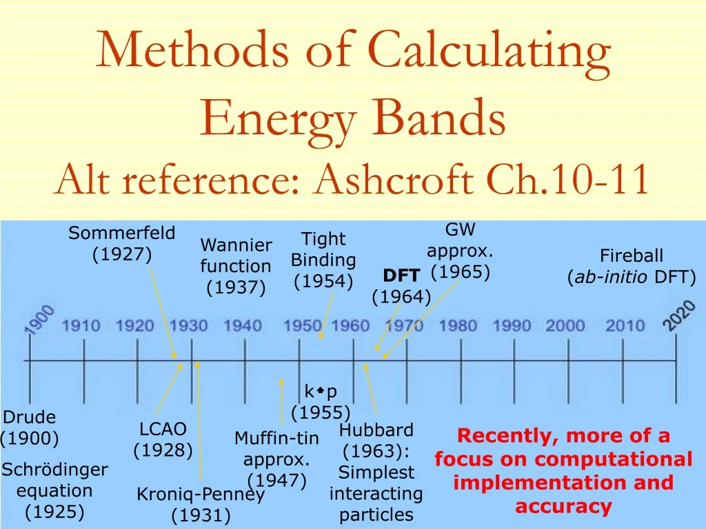
Methods of Calculating Energy BandsAlt reference: Ashcroft Ch.10-11 GW approx. (1965) Sommerfeld (1927) Tight Binding (1954) Wannier function (1937) Fireball (ab-initio DFT) DFT (1964) kp (1955) Drude (1900) LCAO (1928) Hubbard (1963): Simplest interacting particles Recently, more of a focus on computational implementation and accuracy Muffin-tin approx. (1947) Schrödinger equation (1925) Kroniq-Penney (1931)
The Independent Electron (e-) Approximation & Sch. Equation • An independent SE for each e- is simplification • The ind. e- approx. however doesn’t ignore all • U(r)=periodic potential + periodic interactions • To know U(r) with interactions, you need • To know , you need U(r) What to do? • Guess U(r), use to solve Then what? • Use to get better guess of U(r), repeat same
Generalizations to all Methods • Except with the simplest 1D examples, the S. E. cannot be solved exactly • All methods require approximations • And high speed computing! • Thus the type of approximations people have tried has been limited by computing techniques and computing power • Focus on higher energy bands as tight binding is pretty good for lower bands
Hexagonal lattice The Cellular Method (1934) • First iterative approach was the cellular method by Wigner and Seitz (know that name?) • Since we have periodicity, it is enough to solve the S.E. within a single primitive cell Co • The wavefunction in other cell is then • is a sum over spherical harmonics, need BCs • Computationally challenging to solve B.C.s • Results in potential with discontinuous derivative at cell boundary
Muffin-tin potential Solves both complaints of the last method: One way to make sure continuous is set to 0! U(r)=V(|r-R|), when |r-R| ro(the core region) =V(ro)=0,when |r-R| ro(interstitial region) rois less than half of the nearest neighbor distance Of course you are just moving your discontinuous derivative problem, but maybe to better spot?
How to deal with a discontinuous derivative (but continuous ) Best to use variational principle rather than S.E. E[k] is the energy of (k) of the level k Drawback: Different starting potentials can give different results
Two methods use the muffin tin potential Augmented Plane-Wave method (APW) • In the interstitial region k,=eikr • In the atomic region, k, satisfies S.E. • Only k dependence is in the interstitial region • In interstitial region: • Thousands of APWs can be used
Another approach using Muffin tin • The other method is called the Green’s function approach or the Korringa, Kohn, and Rostoker (KKR) method • Formulation seems very different, but it has been established that the methods yield the same results using the same potential
Orthogonalized plane wave method (OPW) • Good if don’t want a doctored potential • Orthogonalized plane waves defined as: • Core levels needed (generally tight binding) • Constants bc determined by orthogonality • This implies • Second term small in interstitial region • So close to a plane wave in interstitial region
Pseudopotential Method • Began as an extension of OPW • If we act H on • In the outer region, this gives ~ free energy • What goes on in core is largely irrelevant to the energy, so let’s just ignore it U(r)=0 , when r Re (the core region) =-e2/r,when r Re (interstitial region)
Pseudopotential Method • Calculation of band structure depends only on the Fourier components of the pseudopotential at the reciprocal lattice vectors (edges of the BZ). • Usually, only a few values of U are needed • Constants from models or fits to optical measurements of reflectance and absorption • Great predictive value for new compounds • Often possible to calculate band structures, cohesive energy, lattice constants and bulk moduli from first principles
Nearly free e-’s • Large overlap • Wave functions ~ plane waves • Assume energy is unchanged and solve for 1st order correction Tight-binding/LCMO • Assume some electrons indep. of each other • Linear combination of • Wannier functions = unperturbed atomic orbital k·p Theory • Useful for understanding interactions between bands • Critical points of BZ have specific properties. • If critical point energies are known, treat nearby points as critical energy plus perturbation Pseudopotential Method includes Coulomb repulsion & Pauli exclusion. No exact way to calculate V(r), guess and iterate. Valence bands->charge density=ѱ*ѱ->V’ Density functional theory (DFT) takes into account Coulomb, exchange and correlation energies of electrons. Guess and iterate. Gives good bandstructure.
k○p Theory • Most holes (electrons) spend most of their time near the top (bottom) of the valence (conduction) band so properties nearby these points important
k○p Theory • Most holes (electrons) spend most of their time near the top (bottom) of the valence (conduction) band so properties nearby these points important • Based on perturbation theory • V~ is the periodic potential (of the lattice), and VU is the confinement potential • V0 and x0 are some arbitrary positive constants. If VU is small, then the solutions to the S.E. are of the Bloch form:
Essense of k○p Theory Reference in notes Plug Bloch into S.E. After lots of manipulation: When we plug in the Bloch wavefunction, we can write the Schrodinger equation in this form. E’k
Nearly free e-’s • Large overlap • Wave functions ~ plane waves • Assume energy is unchanged and solve for 1st order correction Tight-binding/LCMO • Assume some electrons indep. of each other • Linear combination of • Wannier functions = unperturbed atomic orbital k·p Theory • Useful for understanding interactions between bands • Critical points of BZ have specific properties. • If critical point energies are known, treat nearby points as critical energy plus perturbation Pseudopotential Method includes Coulomb repulsion & Pauli exclusion. No exact way to calculate V(r), guess and iterate. Valence bands->charge density=ѱ*ѱ->V’ Density functional theory (DFT) takes into account Coulomb, exchange and correlation energies of electrons. Guess and iterate. Gives good bandstructure.
Basics of DFT-LDA (+U) • DFT’s failures: Materials containing localized d and f electrons whose contributions to exchange and correlation are not accurately computed in the commonly used local density approximation. • Most basic fix is LDA+U, where to the DFT functional is added an orbital-dependent interaction term characterized by an energy scale U, the screened Coulomb interaction between the correlated orbitals. Success = the high temperature superconducting cuprates. • LDA+U’s notable failures. While there are exceptions, it is not expected to adequately describe a system which is not a good insulator.
Dynamical Mean Field Theory (Tudor) • DMFT (or LDA+DMFT) goes beyond LDA+U by allowing the interaction potential of the correlated orbitals to be energy (frequency) dependent. • This frequency dependent potential, or self-energy, is computed for the correlated orbitals only using many-body techniques within an accurate impurity solver. • This calculation can be done as accurately as one desires, and it is significantly cheaper in CPU time than solving a full many-body problem


