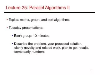
Parallel Algorithms II
Parallel Algorithms II. Topics: matrix and graph algorithms. Solving Systems of Equations. Given an N x N lower triangular matrix A and an N-vector b , solve for x , where A x = b (assume solution exists) a 11 x 1 = b 1 a 21 x 1 + a 22 x 2 = b 2 , and so on….

Parallel Algorithms II
E N D
Presentation Transcript
Parallel Algorithms II • Topics: matrix and graph algorithms
Solving Systems of Equations • Given an N x N lower triangular matrix A and an N-vector • b, solve for x, where Ax = b (assume solution exists) • a11x1 = b1 • a21x1 + a22x2 = b2 , and so on…
Equation Solver Example • When an x, b, and a meet at a cell, ax is subtracted from b • When b and a meet at cell 1, b is divided by a to become x
Complexity • Time steps = 2N – 1 • Speedup = O(N), efficiency = O(1) • Note that half the processors are idle every time step – • can improve efficiency by solving two interleaved • equation systems simultaneously
Inverting Triangular Matrices • Finding X, such that AX = I, where A is a lower triangular • matrix • For each row j, A xj = ej , where ej is the jth unit vector • (0,…, 0, 1, 0,…, 0) and xj is the jth row of matrix X • Simple extension of the earlier algorithm – it can be • applied to compute each row individually
Solving Tridiagonal Matrices • Can be solved recursively with odd-even reduction
Odd-Even Reduction • For each odd i, the corresponding equation Ei is • represented as: • This equation is substituted in equations Ei-1 and Ei+1 • Therefore, equation Ei-1 now has the following unknowns: • xi-1, xi+1, xi-3, (note that i is odd) • We now have N/2 equations involving only even unknowns • – repeat this process until there is only 1 equation with 1 • unknown – after computing this unknown, back-substitute • to get other unknowns
The Algorithm • The ithleaf receives the inputs ui, di, li, and bi • Each leaf sends its values to both neighboring processors • (purple sideways arrows) and every even leaf computes • the u, d, l, and b values for the second level of equations • These values are sent to the next higher level (upward • purple arrows) • After the root computes the value of xN, it is propagated • down and to the sides until all xi are computed (green • arrows)
Gaussian Elimination • Solving for x, where Ax=b and A is a nonsingular matrix • Note that A-1Ax = A-1b = x ; keep applying transformations • to A such that A becomes I ; the same transformations • applied to b will result in the solution for x • Sequential algorithm steps: • Pick a row where the first (ith) element is non-zero and normalize the row so that the first (ith) element is 1 • Subtract a multiple of this row from all other rows so that their first (ith) element is zero • Repeat for all i
Sequential Example 2 4 -7 x1 3 3 6 -10 x2 = 4 -1 3 -4 x3 6 1 2 -7/2 x1 3/2 3 6 -10 x2 = 4 -1 3 -4 x3 6 1 2 -7/2 x1 3/2 0 0 1/2 x2 = -1/2 -1 3 -4 x3 6 1 2 -7/2 x1 3/2 0 0 1/2 x2 = -1/2 0 5 -15/2 x3 15/2 1 2 -7/2 x1 3/2 0 5 -15/2 x2 = 15/2 0 0 1/2 x3 -1/2 1 2 -7/2 x1 3/2 0 1 -3/2 x2 = 3/2 0 0 1/2 x3 -1/2 1 0 -1/2 x1 -3/2 0 1 -3/2 x2 = 3/2 0 0 1/2 x3 -1/2 1 0 -1/2 x1 -3/2 0 1 -3/2 x2 = 3/2 0 0 1 x3 -1 1 0 0 x1 -2 0 1 0 x2 = 0 0 0 1 x3 -1
Algorithm Implementation • The matrix is input in staggered form • The first cell discards inputs until it finds • a non-zero element (the pivot row) • The inverse r of the non-zero • element is now sent rightward • r arrives at each cell at the same • time as the corresponding • element of the pivot row
Algorithm Implementation • Each cell stores di = r ak,I – the value for the normalized pivot row • This value is used when subtracting a multiple of the pivot row from other rows • What is the multiple? It is aj,1 • How does each cell receive aj,1 ? It is passed rightward by the first cell • Each cell now outputs the new values for each row • The first cell only outputs zeroes and these outputs are no longer needed
Algorithm Implementation • The outputs of all but the first cell must now go through the remaining • algorithm steps • A triangular matrix of processors efficiently implements the flow of data • Number of time steps? • Can be extended to compute the inverse of a matrix
Implementation on 2d Processor Array Row 3 Row 2 Row 1 Row 3 Row 2 Row 3 Row 1 Row 1/2 Row 1/3 Row 1 Row 2 Row 2/3 Row 2/1 Row 2 Row 3 Row 3/1 Row 3/2 Row 3 Row 1 Row 2 Row 1 Row 3 Row 2 Row 1
Algorithm Implementation • Diagonal elements of the processor array can broadcast • to the entire row in one time step (if this assumption is not • made, inputs will have to be staggered) • A row sifts down until it finds an empty row – it sifts down • again after all other rows have passed over it • When a row passes over the 1st row, the value of ai1 is • broadcast to the entire row – aij is set to 1 if ai1 = a1j = 1 • – in other words, the row is now the ith row of A(1) • By the time the kth row finds its empty slot, it has already • become the kth row of A(k-1)
Algorithm Implementation • When the ith row starts moving again, it travels over • rows ak (k > i) and gets updated depending on • whether there is a path from i to j via vertices < k (and • including k)
Title • Bullet