Download
1 / 14
140 likes | 338 Vues
The Diminishing Rhinoceros & the Crescive Cow. Exploring, Organizing, and Describing, Qualitative Data. File Information: 14 Slides To Print : You may need to save this to your p: drive or jump drive before printing.Set PRINT WHAT to Handouts.

E N D
The Diminishing Rhinoceros & the Crescive Cow Exploring, Organizing, and Describing, Qualitative Data • File Information: 14 Slides • To Print : • You may need to save this to your p: drive or jump drive before printing.Set PRINT WHAT to Handouts. • Under HANDOUTS select the number of slides per page. A sample of the layout on a page appears to the right. • To change the orientation of the printing, select the PREVIEW button (lower left) and then the Orientation option on the Print Preview menu.
Essentials:Qualitative Data(Be able to address the following.) • Characteristics of qualitative variables. • Building a qualitative frequency table. • Appropriate charts/graphs for qualitative data (and how to make them).
Exploring, Organizing, and Describing Data Before beginning to analyze data, it is important to know three things: 1. Did the data come from a sample or a population? 2. Are the data qualitative or quantitative? 3. In what measurement scale are the data reported? Knowing the characteristics of a variable allows one to select appropriate presentation formats and analysis procedures.
Important Characteristics of a Data Set • Center – an “average” value that indicates where the middle of the data is located. For qualitative data the “center” is represented by the mode, or most frequently occurring value. • Variation – a measure of the amount that the values vary among themselves. • Distribution – the “shape” of the distribution of data. • Outliers – values that are far away from the majority of values. • Time – changing characteristics of data over time.
FREQUENCYDISTRIBUTIONS • A Frequency Distribution represents the range over which a variable’s values occur. For qualitative data the distribution is represented by the categories (values) of the variable. • A Qualitative Frequency Table lists the categories (values) of a variable, along with the frequencies (counts) of the number of values that fall into each category and what portion of all values the category frequency represents, known as the relative frequency. In addition, for ordinal data, a frequency table may show cumulative frequencies and cumulative relative frequencies. • Frequency Tables are derived from RAW DATA through the use of a TALLY process.
Qualitative Frequency Distributions • Qualitative or Categorical Frequency Distributions present categorical data, such as gender, hair color, or military rank. • Each category of the variable is presented along with the frequency of its occurrence and a relative frequency.
Building and Displaying a Qualitative Frequency Distribution(Nominal Data) START HERE: Data: Tally (count) occurrences of each category of the item. Blue: 11111 11111 = 10 Brown: 11111 11111 11 = 12 Green: 11111 11111 1 = 11 Orange: 111 = 3 Red: 11111 111 = 8 Yellow: 11111 11111 111 = 13 Next build the table: List the values of the variable (here color) followed by columns for the frequency of occurrence and the relative frequency Relative freq. = the number of a category/total number of items. For, example, the relative frequency of green candies out of all 57 candies is 11/57 = .193 NOTE: For ordinal data add cumulative frequency and cumulative relative frequency columns as with quantitative tables – example on next slide.)
Variations on a Qualitative Frequency Table The table below presents the same m&m’s data, but in slightly different format. The relative frequency has been replaced by the percent of candies a given color is of all candies. A percentage is equal to the relative frequency * 100. Because of the “ordering” characteristic of ordinal data, two additional columns, cumulative frequency (cf) and cumulative relative frequency (crf), are added to a table.
Bar Chart • The Bar Chart is a commonly used chart for the presentation of qualitative, categorical data. Within a bar chart there will be a bar for each value of the variable. The bar can represent frequency data or relative frequency data. • In a bar chart the bars do not touch and are equal in width. • The height of a bar represents the frequency or relative frequency of the value. BEWARE: Bar Charts and Histograms (used for quantitative data) look similar, but are actually quite different in structure. Knowing what type of data you are working with will lead you to the correct chart type.
Bar Chart Variations: Bar Charts may be used to compare data. A Stacked Bar Chart will divide each bar by some other categorical variable. A Clustered Bar Chart (side by side) will provide separate bars for a variable across the values of a second variable. Clustered Bar Charts: Below are two clustered bar charts. Both depict information regarding the number of houses sold by month in three cities. The bar chart on the left shows where sales occurred and is based upon a count. Dallas experienced far more house sales in a selected month than either other city. In contrast, the bar chart on the right is based upon relative frequency. It shows for each city what portion (rel. freq.) of its total sales occurred each month. Stacked Bar Chart: Below the variable month is sub-divided by the location of the houses sold during the specified months. Count based: Total Sales for a Month. Rel. Freq. based: Portion of total sales for a city.
Pareto Chart A Pareto Chart is similar to a bar chart, except the categories appear from most frequent to least frequent (left to right). Note that there are two y-axes. One for counts and the other for corresponding percentages. In some instances a pareto chart will contain a cumulative frequency line, which represents the summed frequencies from left to right. As a separate chart the cumulative frequency line is called an Ogive (pronounced with a long “i” – Oj-Ive). Ogive -
Graphing Qualitative Data Sets Pie Chart A circle is divided into sectors that represent categories. The area of each sector is proportional to the frequency of each category. Source: Larson/Farber 4th ed.
Pie Chart Pie Charts present qualitative data or grouped quantitative data. To determine the size of each slice, first find the relative frequency for a value or category. Then multiply the relative frequency times 360o. The result will be the portion of the circle’s circumference that will represent the category. Example: 11 green candies represent .193 (or 19.3%) of all candies. Multiply 360o * .193 = 69.48o, which is the length of the arc on the circumference representing green candies. NOTE: Arc degrees are not included on pie charts. Arc = 69.480