Download
1 / 37
370 likes | 625 Vues
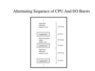
Alternating Sequence of CPU And I/O Bursts. Histogram of CPU-burst Times. CPU Scheduler. Selects from among the processes in memory that are ready to execute, and allocates the CPU to one of them. CPU scheduling decisions may take place when a process:

E N D
CPU Scheduler • Selects from among the processes in memory that are ready to execute, and allocates the CPU to one of them. • CPU scheduling decisions may take place when a process: 1. Switches from running to waiting state. 2. Switches from running to ready state. 3. Switches from waiting to ready. 4. Terminates. • Scheduling under 1 and 4 is nonpreemptive. • All other scheduling is preemptive.
Dispatcher • Dispatcher module gives control of the CPU to the process selected by the short-term scheduler; this involves: • switching context • switching to user mode • jumping to the proper location in the user program to restart that program • Dispatch latency – time it takes for the dispatcher to stop one process and start another running.
Scheduling Criteria • CPU utilization – keep the CPU as busy as possible • Throughput – # of processes that complete their execution per time unit • Turnaround time – amount of time to execute a particular process • Waiting time – amount of time a process has been waiting in the ready queue • Response time – amount of time it takes from when a request was submitted until the first response is produced, not output (for time-sharing environment)
Optimization Criteria • Max CPU utilization • Max throughput • Min turnaround time • Min waiting time • Min response time
First-Come, First-Served (FCFS) Scheduling ProcessBurst Time P1 24 P2 3 P3 3 • Suppose that the processes arrive in the order: P1 , P2 , P3
P1 P2 P3 0 24 27 30 The Gantt Chart for the schedule is: • Waiting time for P1 = 0; P2 = 24; P3 = 27 • Average waiting time: (0 + 24 + 27)/3 = 17
P2 P3 P1 0 3 6 30 FCFS Scheduling (Cont.) Suppose that the processes arrive in the order P2 , P3 , P1 . • The Gantt chart for the schedule is: • Waiting time for P1 = 6;P2 = 0; P3 = 3 • Average waiting time: (6 + 0 + 3)/3 = 3 • Much better than previous case. • Convoy effect short process behind long process
Shortest-Job-First (SJR) Scheduling • Associate with each process the length of its next CPU burst. Use these lengths to schedule the process with the shortest time. • Two schemes: • nonpreemptive – once CPU given to the process it cannot be preempted until completes its CPU burst.
Shortest-Job-First (SJR) Scheduling • preemptive – if a new process arrives with CPU burst length less than remaining time of current executing process, preempt. This scheme is know as the Shortest-Remaining-Time-First (SRTF). • SJF is optimal – gives minimum average waiting time for a given set of processes.
Example of Non-Preemptive SJF Process Arrival TimeBurst Time P1 0.0 7 P2 2.0 4 P3 4.0 1 P4 5.0 4
P1 P3 P2 P4 0 3 7 8 12 16 Example of Non-Preemptive SJF • Average waiting time = (0 + 6 + 3 + 7)/4 - 4
Example of Preemptive SJF Process Arrival TimeBurst Time P1 0.0 7 P2 2.0 4 P3 4.0 1 P4 5.0 4
P1 11 16 0 2 4 5 7 Process Arrival TimeBurst Time P1 0.0 7 Executes for two seconds.
P1 P2 P3 P2 P4 P1 11 16 0 2 4 5 7 Process Arrival TimeBurst Time P1 0.0 7 P2 2.0 4 P2 Remainder = 4. P1 Remainder = 5. Result: P1 preempted at time 2.
P1 P2 P3 P2 P4 P1 11 16 0 2 4 5 7 Process Arrival TimeBurst Time P1 0.0 7 P2 2.0 4 P3 4.0 1 P1: 5 P2: 2 P2 Preempted. P3 completes at time 5. P3: 1
Process Arrival TimeBurst Time P1 0.0 7 P2 2.0 4 P4 5.0 4 P1: 5 P2: 2 P4: 4
P1 P2 P3 P2 P4 P1 11 16 0 2 4 5 7 P2 Completes at time 7. P1: Remaining time of 5. P4: Remaining time of 4.
P1 P2 P3 P2 P4 P1 11 16 0 2 4 5 7 P1: Remaining time of 5. P4: Remaining time of 4.
Determining Length of Next CPU Burst • Can only estimate the length. • Estimate made based on some sort of statistic of historical behavior. • Assume BL2 == BL1 (Next same as last). • Take mean of last n burst lengths. • Exponential average of previous bursts.
Scheduling in Batch Systems Three level scheduling
Memory Scheduler • Decisions based on for example: • Time since swapped out. • Amount of CPU time allocated so far. • How large. • How important.
Admission Scheduler • Based on “degree of multiprogramming” • Process mix.
Priority Scheduling • A priority number (integer) is associated with each process • The CPU is allocated to the process with the highest priority (smallest integer highest priority). • Preemptive • nonpreemptive • SJF is a priority scheduling where priority is the predicted next CPU burst time. • Problem Starvation – low priority processes may never execute.
Priority Scheduling • Solution Aging – as time progresses increase the priority of the process. • Unix has mechanism for user to lower their priority through the nice system call. Never used.
Scheduling for Interactive Systems: Round Robin (RR) • Each process gets a small unit of CPU time (time quantum), usually 10-100 milliseconds. After this time has elapsed, the process is preempted and added to the end of the ready queue. • If there are n processes in the ready queue and the time quantum is q, then each process gets 1/n of the CPU time in chunks of at most q time units at once. No process waits more than (n-1)q time units. • Performance • q large FIFO • q small High overhead: Must be large with respect to context switch, otherwise overhead is too high.
Scheduling in Interactive Systems • Round Robin Scheduling • list of runnable processes • list of runnable processes after B uses up its quantum
How long should the quantum be? • quantum too short • Assume switch time = 5ms and quantum = 20ms: Wasted time = 5/(5+20) = 20% • quantum too long: e.g., switch time = 5ms, quantum = 200ms: Wasted time = 5/(5+200) = approx. 2% but if have 100 processes, response time for 200th is pretty bad. This is the quantum Linux uses.
Multilevel Queue • Ready queue is partitioned into separate queues:foreground (interactive)background (batch) • Each queue has its own scheduling algorithm, foreground – RRbackground – FCFS
Multilevel Queue • Scheduling must be done between the queues. • Fixed priority scheduling; (i.e., serve all from foreground then from background). Possibility of starvation. • Time slice – each queue gets a certain amount of CPU time which it can schedule amongst its processes; i.e., 80% to foreground in RR • 20% to background in FCFS
Multilevel Feedback Queue • A process can move between the various queues; aging can be implemented this way. • Multilevel-feedback-queue scheduler defined by the following parameters: • number of queues • scheduling algorithms for each queue • method used to determine when to upgrade a process • method used to determine when to demote a process • method used to determine which queue a process will enter when that process needs service
Example of Multilevel Feedback Queue • Three queues: • Q0 – time quantum 8 milliseconds • Q1 – time quantum 16 milliseconds • Q2 – FCFS • Scheduling • A new job enters queue Q0which is servedFCFS. When it gains CPU, job receives 8 milliseconds. If it does not finish in 8 milliseconds, job is moved to queue Q1. • At Q1 job is again served FCFS and receives 16 additional milliseconds. If it still does not complete, it is preempted and moved to queue Q2.