Collision Recognition System Using Video Analysis for Vehicle Trajectories
500 likes | 630 Vues
This project aims to design a system that recognizes potential vehicle collision trajectories using video footage captured from a rear-facing camera. The objectives include alerting drivers to possible dangers, allowing for timely reactions. The proposed algorithm, developed in MATLAB, focuses on 3D world reconstruction and employs advanced feature detection methods, including ASIFT. By analyzing changes in dynamic features, the system differentiates between static and moving objects, enhancing safety for drivers through effective pre-collision alerts.

Collision Recognition System Using Video Analysis for Vehicle Trajectories
E N D
Presentation Transcript
Collision recognition from a videopart A Students: AdiVainiger, EyalYaacoby Supervisor: NetanelRatner Laboratory of Computer Graphics & Multimedia Electrical Engineering faculty, Technion Semester: Winter 2012
Objective • Design a system with two main roles: • Recognize possible collision trajectories by vehicles, using a video taken from a camera directed toward the rear of the direction of driving • Alert the user so he can react accordingly • Part A goal: Design an algorithm for the system using MATLAB • Without taking into account real-time constraints
Related Work • Mobileye[1] • Israeli company that developed an alerting system for car drivers • Front and rear cameras • Algorithm - based on changes of the vehicles’ width in the scene. • Our goal is similar but designed differently • Full reconstruction of the 3D world - enables accurate results.
Feature Detection and Matching • Interest points detection • LaplacianPyramids (computed by DoG) • Interest points are the extrema in scale-space (x,y;s) [2] [3]
Feature Detection and Matching • SIFT • Image descriptor - for each interest point • Grid – 4x4 • Scale Normalization – by level in pyramid • Orientation Normalization – by largest gradient • Gradient histogram per cell • By pixel gradient • 8 quantized directions • Descriptor size 4x4x8 = 128 dimensions [4]
Feature Detection and Matching • SIFT • Matching • Closest neighbor by Euclidean distance between descriptors [5]
Feature Detection and Matching • ASIFT • Affine extension of SIFT • ASIFT is much more accurate, gives more features • ASIFT is slower than SIFT (~50x) • We’ve used ASIFT for accuracy reasons
Perspective Projection • Camera - Pinhole model • (X0, Y0 , Z0) (U0, V0)
Perspective Projection • Matrix Representation • Translation and Rotation • Projection • Ideal camera calibration matrix • Real camera calibration matrix • Final model of camera transformation • Using homogenous coordinates (Xf, Yf, Zf) = pinhole coordinates normalization
3D Reconstruction • Fundamental Matrix • Represents transformation between two frames • x - 2D point in frame 1 (projection of X in 3D world) • x‘ – 2D point in frame 2 (projection of same X) • Fx – epipolarline on frame 2 • Also the projection of the epipolar plane on frame 2 • Geometric constraint • Meaning: x‘ must be on the line Fx • rank(F) = 2 [6] X [6] l = Fx x x’
3D Reconstruction • Fundamental Matrix • Estimating using RANSAC • Generating many hypotheses (e.g. 500) • Choosing 8 random points • Estimating F using these 8 points (eight point algorithm) • Choosing the best hypothesis • Minimizes the sum of error for all points
3D Reconstruction • Estimating transformation between frames • Essential Matrix E • Similar to fundamental matrix, with normalized coordinates • Can be defined as • Satisfies • t,R - translation and Rotation between the two frames • Using SVD for E we get 4 Options • R is determined up to π degrees rotation (= 2 options) • t is determined up to sign (= 2 options)
3D Reconstruction • Triangulation • We now know the relative translation and Rotation (R’,t’) between the two frames • We set the first camera to be at the origin : • We can draw two lines in 3D space: from each interest point to camera center • Ideally, these two lines should intersect at the real 3D point • Realistically, due to noise, the two lines don’t intersect • We approximate by linearization and error minimization • is the reconstructed point [7]
Our Implementation • Feature Detection & Matching using ASIFT Feature Detection & Image Descriptors Frame 1 Matches Matching Interest Points Feature Detection & Image Descriptors Frame 2
Our Implementation • 3D Reconstruction [*] Assuming the Calibration Matrix is known • Using the methods explained earlier • Out of 4 solutions, we eliminate 3 impossible ones: • Angular difference between the frames is larger than 180° • The reconstructed points are behind the camera 3D Reconstructed points Matches Triangulation [*] Estimating transformation between frames Fundamental Matrix
Recognition and DifferentiationBetween Static and Moving Objects • For N Frames creating N-1 reconstructions • Each reconstruction is between frames i and i-5 • Reconstructions Matching • For each 3D point in the newest reconstruction , finding the closest points in N-2 earlier reconstructions Dynamic Feature Points Variance Calculation for each point Reconstructions Matching Static Feature Points 3D Reconstructed points 3D Reconstructed points 3D Reconstructed points 3D Reconstructed points N-1
Recognition and DifferentiationBetween Static and Moving Objects • Indicators • Dynamic points have greater epi-polar error • Dynamic points have higher variance (for each point and its matches) • Variance Normalization • We need to normalize by the expected error • Distance from camera - • Angle between triangulation lines - • Setting some threshold for each indicator • Points that have variance above the threshold – are Dynamic Point that have variance below the threshold – are Static Dynamic Feature Points Variance Calculation for each point Reconstructions Matching Static Feature Points 3D Reconstructed points 3D Reconstructed points 3D Reconstructed points 3D Reconstructed points N-1
Collision Detection • Reconstruction by static points • More accurate reconstructions of the dynamic points than the ones we had • Estimate dynamic points scattering • On collision course, the reconstructed points are widely scattered • Counting how many balls are needed to cover all the points If greater than some threshold (e.g. 10), we assume some object is on a collision course Estimate dynamic points scattering Is there collision? Static Points Static Points שחזור העולם התלת-ממדי על פי הנקודות הסטטיות בלבד Static Points שחזור העולם התלת-ממדי על פי הנקודות הסטטיות בלבד Static Feature Points Reconstruction of the Dynamic points N-1 N Static Points Static Points Static Points Dynamic Feature Points N-1 N שחזור העולם התלת-ממדי על פי הנקודות הסטטיות בלבד שחזור העולם התלת-ממדי על פי הנקודות הסטטיות בלבד Estimating Fundamental Matrix by the Static points
3D Synthetic World • Objects in picture are represented by trees (static objects) and cars (moving objects) • Each “tree” is a blue box • Each “car” is a green box • From each object we randomlychoose a predetermined number of 3D points (~64) • Vehicle represented by a moving camera • The camera is a pink pyramid • The camera has an angle relative to the moving direction • Takes a picture every 1/20 second • The interest points are the perspective projection of the chosen 3D points • Gaussian noise is added to the 2D projected points
3D Synthetic World • Scenarios • Creation - We chose 6 scenarios for testing – where the direction of the car changes. e.g. • Collision direction : • Same direction:
3D Synthetic World • Scenarios Reconstruction Results • Collision direction : • Same direction :
3D Synthetic World • Collision Detection Results : • Conclusions : • Setting the threshold to 10, we can correctly identify collision • 2% false negatives on collision scenario (collision but no alarm) • 12% false positives on the worst scenario (alarm but no collision)
Synthetic Results • Tests - The error in 3D reconstruction by noise • Changing different parameters • Reconstruction based on Static vs. Static & Dynamic points • The error is significantly larger when dynamic points are included • Conclusion:Separation between static and dynamicobjects is crucial for a reliable 3D reconstruction • Implementation:We reconstruct the world using basedon the static points only after separation
Synthetic Results • Frame rate : 1 - 20 per sec • The error is very largewhen comparingconsecutive frames • Conclusion: Reconstruction should be based on frames farther apart. The bigger difference between frames makes the noise less significant. • Implementation: Reconstruction is based on frames that are 5 frames apart
Synthetic Results • Camera angle – 0 °-90° • The camera angle significantlyaffects the error - the larger theangle*, the smaller the error * relative to the forward direction • Conclusion: The camera angle creates a larger difference between frames, so the noise has less affect • Implementation: The camera should be positioned in an angle relative to the forward direction
Synthetic Results • Trees position – distance from camera : 7-31 meters • The tree position significantlyaffects the error – the farther the tree , the less accurate the result • Number of interest points of each object : 32-128 • The more points – the merrier
Movie Results • Two movie types • Camera on cyclist’s helmet • Camera on Roomba
Movie Results • Calibration • Using an external toolbox for Matlab • Getting the calibration matrix K • Fixing radial distortion using an external algorithm
Movie Results • Feature detection and matching • Dynamic points • Rolling shutter caused distortion due to the vibrations of Roomba • ASIFT misses the dynamic points in majority of movies • Solution: manual feature matching (using cpselect tool)
Movie Results • Estimating Ego – motion using essential matrix • Rotation – • Camera was fixed to the robot during the shooting • Expecting rotation ~ 0 • The result was as expected • Translation – • The translation size was determined by us • Expecting angle between x-y axis 30° • The result was around 25° • Conclusion – • Ego motion is estimated correctly • Thus we assume Fundamental matrix and calibration of the camera are correct.
Movie Results • Reconstruction of the world
Movie Results • Recognition and Differentiation Between Static and Moving Objects • Epi-polar error • The epi-polar error does not correlate well with the expected result • We get a lot of static points with a high error and some dynamic points with a low error • We have decided not to use it
Movie Results • Recognition and Differentiation Between Static and Moving Objects • Variance • Measuring variance among several 3D reconstructions • Distant objects have a high variance • Using un-normalized variance, We cannot distinguish between distant and dynamic points
Movie Results • Recognition and Differentiation Between Static and Moving Objects • Normalized Variance • 1) Distance from camera - • Threshold = 0.05 • 2) Angle between triangulation lines – • Threshold = 3.3e-6 • We get better results than previous methods • Still, there are scenes where it doesn’t work as expected
Summary and Conclusions • There were several major problems in the project • 1) Matching features of moving objects • Doesn’t work, largely due to the vibrations in video capturing • In a real scenario, we expect much less vibrations • 2) Classifying static and moving objects • Even the best algorithm fails on many cases • A form of tracking (e.g. KLT) can help solve this problem • 3) Long running time (~3 minutes per frame) • Most of the time is spent on ASIFT • A faster feature matching algorithm can resolve this
Summary and Conclusions • Further research • Using a tracking algorithm (e.g. KLT) • Should solve the matching problem • Much better classification between static and moving objects • Identifying vehicles • An algorithm that recognizes vehicles (e.g. Viola and Jones) • Allows focusing only on interesting objects instead of the entire frame • Accurate triangulation • Using the full polynomial error estimation instead of the linear approximation
Thank you for Listening
Appendix A : Essential Matrix • SVD for essential matrix • The SVD can be represented in 2 ways: • Overall: 4 options
Appendix B : Triangulation • Approximation of the reconstruction of the 3D point in presence of noise • The homogeneous interest points in frames 1 and 2 should satisfy the equations: • Due to noise there is no solution - as • We would like to minimize , s.t • The solution is the singular vector with the lowest singular value out of the SVD of A .
Static Point Reconstruction Appendix C : Static &Moving Objects Dynamic Point Reconstruction Low Variance High Variance
Appendix D: Collision Detection • Collision course • On a collision course,the lines between the camera centers and theobject are almostparallel • Thus, the reconstructions will be very distant from one another • We identify this by measuring dynamic points scattering • Note - This property is not unique to collision courses
Appendix E: Collision Detection • Clustering Algorithm • We want to count how many balls are needed to cover all the reconstructed points • While there are points remaining: • Choose a random point • Draw a ball around it • Remove all points inside the ball • The number of balls used is the result of the algorithm • This is used as a metric for points scattering • We implemented a k-medoids algorithm • Produced almost the same results, but performance was much worse – we chose the above random algorithm [8]
Appendix F: Triangulation ambiguity • Uncertainty of reconstruction depends on the angle between the triangulation rays • Reconstructed points has more ambiguity along the ray as the rays become more parallel • Forward\ backward motion – rays almost parallel , thus reconstruction is even more weak Less ambiguity Higher ambiguity
References • [1] E.Dagan, O.Mano, G. P. Stein, A.Shashua, Forward Collision Warning with a Single Camera, 2004 • [2] Mikhail Sizintsev, http://www.cse.yorku.ca/~sizints • [3] http://www.scholarpedia.org/article/File:Strandvagen2-Laplace1500pts.png • [4] David G. Lowe, "Distinctive image features from scale-invariant keypoints,"International Journal of Computer Vision, 60, 2 (2004), pp. 91-110. • [5] http://www.scholarpedia.org/article/SIFT • [6] http://www.consortium.ri.cmu.edu/projMultiView.php • [7] Hartley and Zisserman, Multiple View Geometry in Computer Vision, 2nd ed. p.311 • [8] http://en.wikipedia.org/wiki/K-medoids