Basic Principles
Introduction to NMMB Dynamics: How it differs from WRF-NMM Dynamics Zavisa Janjic NOAA/NWS/NCEP/EMC , College Park, MD . Basic Principles. Forecast accuracy Fully compressible equations

Basic Principles
E N D
Presentation Transcript
Introduction to NMMB Dynamics: How it differs from WRF-NMM DynamicsZavisa JanjicNOAA/NWS/NCEP/EMC, College Park, MD
Basic Principles • Forecast accuracy • Fully compressible equations • Discretization methods that minimize generation of computational noise and reduce or eliminate need for numerical filters • Computational efficiency, robustness Janjic, Z., and R.L. Gall, 2012: Scientific documentation of the NCEP nonhydrostaticmultiscale model on the B grid (NMMB). Part 1 Dynamics. NCAR Technical Note NCAR/TN-489+STR, DOI: 10.5065/D6WH2MZX. http://nldr.library.ucar.edu/repository/assets/technotes/TECH-NOTE-000-000-000-857.pdf
Nonhydrostatic Multiscale Modelon the B grid (NMMB) • Wide range of spatial and temporal scales (meso to global, and weather to climate) • Built on NWP and regional climate experience by relaxing hydrostatic approximation rather than by extending a cloud model to synoptic scales (Janjic et al., 2001, MWR; Janjic, 2003, MAP) • Further evolution of WRF Nonhydrostatic MesoscaleModel (NMM) (Janjic, 2005, EGU; Janjic & Black, 2007, EGU; Janjic & Gall 2012, NCAR) • Add-on nonhydrostatic module • Easy comparison of hydrostatic and nonhydrostatic solutions • Reduced computational effort at lower resolutions • Pressure based vertical coordinate, nondivergent flow remains on coordinate surfaces
Inviscid Adiabatic Equations Nonhydrostatic pressure Hydrostatic pressure Difference between hydrostatic pressures at surface and top General hybrid coordinate Gas law Constant depth of hydrostatic pressure layer at the top Zero at top and bottom of model atmosphere Hypsometric (not “hydrostatic”) Eq. Increases from 0 to 1 from top to bottom Hydrostatic continuity Eq. Continued …
Inviscid Adiabatic Equations, contd. Integral of nonhydrostatic continuity Eq. Vertical acceleration Third Eq. of motion Momentum Eq. Thermodynamic Eq.
Nonhydrostatic Dynamics Specifics • F, w, e are not independent, no independent prognostic equation for w! • More complex highly implicit numerical algorithm, but no over-specification of w • No computation of 3D divergence • e <<1 in meso and large scale atmospheric flows • Impact of nonhydrostatic dynamics becomes detectable at resolutions <10km, important at 1km.
Discretization Principles • Conservation of important properties of the continuous system aka “mimetic” approach in Comp. Math. (Arakawa 1966, 1972, …; Jacobson 2001; Janjic 1977, 1984, …; Sadourny, 1968, … ; Tripoli, 1992 …) • Nonlinear energy cascade controlled through energy and enstrophy conservation • A number of properties of differential operators preserved • Quadratic conservative finite differencing • A number of first order (including momentum) and quadratic quantities conserved • Omega-alpha term, transformations between KE and PE • Errors associated with representation of orography minimized • Mass conserving positive definite monotone Eulerian tracer advection
Horizontal E grid h v h v h v h v h v h v v h h v h v h d dy v h v h v dx h v h v h
Vertical Coordinate Sangster, 1960; Arakawa & Lamb, 1977
Nonhydrostatic Multiscale Modelon the B grid (NMMB) • Coordinate system and grid • Global lat-lon • Regional rotated lat-lon, more uniform grid size • Arakawa B grid h hh v v h hh v v h hh • Lorenz vertical grid • Pressure-sigma hybrid (Simmons & Burridge 1981, Eckermann 2008) h h hh V dy dx
Layer thicknesses Layer thicknesses Figure 7. Examples of thicknesses of 64 NMMB layers in Pa depending on surface pressure, 1000 hPa (upper left panel), 750 hPa (upper right panel) and 500 hPa (lower left panel). Transition to hydrostatic pressure coordinate occurs at about 300 hPa, and the top of the model atmosphere is at 10 hPa. Cumulative distribution of topography height in medium resolution global NMMB is also shown in 100 m bins (lower right panel). Pressure Pressure ps=750 hPa ps=1000 hPa Layer thicknesses Cumulative topography height 100 m bins Pressure ps=500 hPa
Nonhydrostatic Multiscale Modelon the B grid (NMMB) • Time stepping • No splitting • Adams-Bashforth for horizontal advection of u, v, T (no iterations) and Coriolis force • Crank-Nicholson for vertical advection of u, v, T (implicit) • Forward-Backward (Ames, 1968; Gadd, 1978; Janjic and Wiin-Nielsen, 1977, JAS) fast waves • Implicit for vertically propagating sound waves (Janjic et al., 2001, MWR; Janjic, 2003, MAP, 2011, ECMWF)
WRF NMM Lateral Boundary Conditions • Specified from the driving model along external boundaries • 4-point averaging along first internal row (Mesinger and Janjic, 1974; Miyakoda and Rosati, 1977; Mesinger, 1977) • Upstream advection area next to the boundaries from 2nd internal row • Advection well posed along the boundaries, no computational boundary condition needed • Dissipative • HWRF internal nesting discussed elsewhere
WRF NMM Lateral Boundary Conditions External Boundary h v h v h v h v h v h v h v h v h v h v h v h v h v h v h v h v h v h v h v h v h v h v h v 1st Internal Row, 4 Pt Averaging h v h v h v h v h v h v h v h v h v h v h v h v h v h v h v h v h v h v h v h v h v h v h v Upstream Advection Area h v h v h v h v h v h v h v h v h v h v h v h Domain Interior v h v h v h v h v h v h v h v h v h v h v h v h v h v h v h v h v h v h v h v h v h v h v h v h v h v h v h v h v h v h v h v h v h v h v h v h v h v h v h v h v h v h v h v h v h v h v h v h v h v h v h v h v h v h v h v h v h v h v h v h v h v h v h v h v h v h v h v h v h
Nonhydrostatic Multiscale Modelon the B grid (NMMB) • Regional domain lateral boundaries • Narrow zone with upstream advection, no computational outflow BC for advection • No 4-point averaging, not needed • Blending zone • NMMB internal lateral boundaries addressed elsewhere
upstream advection blending zone outer boundary for wind variables outer boundary for mass variables NMMB Lateral Boundaries • Regional domain lateral boundaries
NMMB Physics • Upgraded NCEP WRF NMM “standard” physical package • RRTM, GFDL radiation • NOAH, LISS land surface models • Mellor-Yamada-Janjic turbulence • Ferrier microphysics • Betts-Miller-Janjic convection • Extensions • NEMS GFS physics • Separate SAS, Zhao, Thompson, GFS PBL, WSM6 ...
Atmospheric Spectrum • Reformulating advection terms from E to B grid was most difficult • False nonlinear energy cascade (Phillips, 1954; Arakawa, 1966 … ; Sadourny 1975; …) major generator of excessive small scale noise • Other computational errors • Historically, problem controlled by: • Removing spurious small scale energy by numerical filtering, dissipation • Preventing excessive noise generation by enstrophy and energy conservation (Arakawa, 1966 …)
Atmospheric Spectrum • Classical paper by Sadourny, 1975, JAS: • Filtering just cosmetics, atmospheric model not needed for “correct” atmospheric spectrum!
Atmospheric Spectrum • Instead (Sadourny, 1975, JAS): • Philosophy built into the design of the compact nonlinear momentum advection schemes for semi-staggered grids (Janjic, 1984, MWR; Janjic, 2004, AMS; Janjic and Gall, 2012, NCAR)
Second order schemes • Formal accuracy does not solve the problem • Blue – Janjic, 1984, MWR; red – controlled energy cascade, but not enstrophy conserving, Arakawa, 1972, UCLA; green – energy and (alternative) enstrophy conserving • Different nonlinear noise levels (green scheme) with identical formal accuracy and truncation error (Janjic et al. 2011, MWR) • Enhanced formal accuracy of well behaved conservative nonlinear advection scheme did not add measurable value to global forecasts in terms of Anomaly Correlation Coefficient. Fourth order schemes 116 days
Anomaly correlation coefficients calculated over the globe averaged over 111 cases for the second order scheme c2 (blue diamonds) and the fourth order scheme c4 (purple squares).
108 -3 105 -5/3 104 103 102 101 103 102 Atmospheric Spectrum Nastrom-Gage (1985, JAS) 1D spectra in upper troposphere and lower stratosphere from commercial aircraft data No spectral gap Transition at few hundred kilometers from –3 to –5/3 slope in the 102-103 km (mesoscale) range Inertial range, 0.01-0.3 m s-1 in the –5/3 range, not to be confused with severe mesoscale phenomena!
● Small scale energy in short regional runs with controlled nonlinear cascade and controlled noise sources, where from? Flat bottom (Atlantic), NMMB, 15km, 32 levels, 48h run (Loops) No Physics With Physics -5/3 -5/3 -3 -3 ● Spectrum in agreement with observed spun-up given physical (or spurious, e.g. sigma) sources on small scales.
Loop, decaying 3D turbulence, Fort Sill storm, 05/20/77. NMM-B, Ferrier microphysics, 1km resolution, 32 levels, 112km by 112km by 16.4km, double periodic, Smagorinsky constant 0.32. Note the hump with active convection Spectrum of w2 at 700 hPa.
Hours 3-4 average decaying 3D turbulence, Fort Sill storm, 05/20/77. NMM-B, Ferrier microphysics, 1km resolution, 32 levels, 112km by 112km by 16.4km, double periodic. Smagorinsky constant 0.32. Spectrum of w2 at 700 hPa. -5/3
Warm bubble, 100 m resolution • 2D very high resolution tests Normalized vertical momentum flux, 400 m resolution Cold bubble, 100 m resolution Full compressible NMM Analytical (Boussinesque) ARPS (Boussinesque) Nonlinear mountain wave 400 m resolution
Convection, 1 km resolution Mountain waves, 8 km resolution
2004 WRF-NMM WRF-NMM WRF-NMM Eta Eta Eta 4km resolution, no parameterized convection Breakthrough that lead to application of “convection allowing” resolution for storm prediction 22nd Conference on Severe Local Storms, October 3-8, 2004, Hyannis, MA.
4 km 1.33 km Observed A difficult tornadic situation from spring 2011, impact of resolution, courtesy of Aligo, Jovic and Ferrier
Hypothetical NMMB Simultaneous Run Global [with Igor & Julia] and NAM [with CONUS nest] Courtesy of DiMego et al. 12 km NAM NMMB 9 km Julia NMMB 4 km NAM-nest NMMB 9 km Igor NMMB 12 km NAM NMMB 27 km Global NMMB 27 km Global NMMB
Meso Scales • Regional NMMB replaced WRF NMM in the NAM slot in 2011 • Hierarchy of nests running simultaneously, 12 km, 6 km, 4 km, 1.33 km (fire weather on the fly) resolutions (DiMego et al.) • Hurricane runs with NMMB using HWRF set-up primarily to test the NMMB infrastructure (initialization, mechanics of nest movements, telescoping and 2-way interactions …)
Summary and Conclusions • Significant improvements of regional forecasts still possible • Unified model offers consistency in applications on various scales and reduced development and maintenance effort and cost • Limits of deterministic forecasting have not been reached yet
Differences between Global and Regional Versions of NMMB Zavisa Janjic, Ratko Vasic, Tom BlackNOAA/NWS/NCEP/EMC, College Park, MD
Differences • Coordinate system • Regional (“basin scale”): rotated lat-lon • Global: lat-lon • Polar boundary condition • Polar filter • Polar points averaging • East-west periodicity
ghost line, mass variables ghost line, wind variables North Pole, mass variables wind variables mass variables Variables near the North Pole • Conservative global polar boundary conditions • Spatial differencing as anywhere else • Polar averaging
Specifying Ghost Line Variables • Change sign of across the pole wind components along the ghost line • No change at scalar points ghost line
Polar Filter • Polar points singular • Convergence of meridians • Coriolis force tends to infinity due to curvature terms • Polar filter • “Decelerator,” tendencies of T, u, v, Eulerian tracers, divergence, dw/dt • Waves in the zonal direction faster than waves with the same wavelength in the latitudinal direction slowed down • No impact on amplitudes of basic variables • Physics not filtered
Polar Filter • Current set-up • Filtering north of 450 N and south of 450 S • At 450 N and 450 S , considered as representative resolution • Can be changed
Physics • Unified model offers consistency in applications on various scales and reduced development and maintenance effort and cost • Unified physics across the scales desirable • Parameterizations depend on scales and have to be differently tuned, but the same parameterization schemes still can be used
Physics • Upgraded NCEP WRF NMM “standard” physical package • RRTM, GFDL radiation • NOAH, LISS land surface models • Mellor-Yamada-Janjic turbulence • Ferrier microphysics • Betts-Miller-Janjic convection • Extensions • GFS physics • Separate SAS, Zhao, Thompson, GFS PBL, WSM6 ...
Data assimilation • Spectral GFS analysis not a good long term choice • GFS analysis even more GFS specific with GFS ensemble cross correlations • Indigenous NMMB analysis needed • Work under way
Computational Considerations • Spherical geometry is an issue, no matter which grid topology is chosen • ~ 50% waste (compared to regional) • Polar filter based on FFT • Serial, nonlocal FFT used • FFT fast, but requires transposition to take advantage of parallel processing • Hindrance for scaling?
Scaling on Zeus • Global, nonhydrostatic, full physics • Easily satisfies NCEP operational requirements • Resolution 1149 x 811 x 64, ~ 24 km • 500 processors, 7.9 wall clock min/day • 4000 processors, 1 year of simulation in < 17 hours, climate studies • Resolution 2305 x 1623 x 64, ~ 12 km • 8 x more work than 1149 x 811 x 64, ~ 24 km • 3600 processors, 7.6 wall clock min/day • 7.2 times more processors for 8 times bigger job in less time! • Operational global ~ 10 km resolution forecasts possible
Scaling • Scaling not critical at present with reasonable resolution and number of cores • Depends on size and shape of sub domains • Slows down with less than 200-250 grid points per core • Parallel FFT now available, presumably will reduce communications significantly
Global Scales • Long verification periods needed to obtain robust scores. • To save on resources and time, a sample of 105 cases over one year at three and a half day intervals (code maintenance, launcher scripts, verification and graphics courtesy of Vasic) • Both 00Z and 12Z initial data equally represented • Sample cases chosen randomly, results should be reasonably representative for a full year population
Global NMMB 1149 x 811 x 64 pts. vs. GFST574 x 64 105 randomly chosen cases from 1 year 500 hPa Height Anomaly Correlation Coefficient vs. forecast time NMMB initialized and verified using GFS analyses and climatology Zeus test Global NMMB 1149 x 811 x 64 pts. vs. GFST574 x 64 105 randomly chosen 00Z and 12Z cases over 1 year Zhao, BMJ, mixed shallow, momentum transport 500 hPa Height Anomaly Correlation vs. forecast time NMMB initialized and verified using GFS analyses and climatology
Global NMMB 1149 x 811 x 64 pts. vs. GFST574 x 64 105 randomly chosen cases from 1 year 500 hPa Height Anomaly Correlation Coefficient vs. forecast time NMMB initialized and verified using GFS analyses and climatology Zeus test Global NMMB 1149 x 811 x 64 pts. vs. GFST574 x 64 105 randomly chosen 00Z and 12Z cases over 1 year Zhao, BMJ, mixed shallow, momentum transport 500 hPa RMSE differences vs. forecast time NMMB initialized and verified using GFS analyses and climatology RMSE difference generally remains within bounds of initial interpolation errors Recent test