An efficient image segmentation algorithm using bidirectional Mahalanobis distance
An efficient image segmentation algorithm using bidirectional Mahalanobis distance. COMMITTEE MEMBERS Dr.Stan Birchfield Dr.Adam Hoover Dr.Brian Dean. MASTERS THESIS By: Rahul Suresh. Thesis overview. Introduction Related work Background theory: Image as a graph

An efficient image segmentation algorithm using bidirectional Mahalanobis distance
E N D
Presentation Transcript
An efficient image segmentation algorithm using bidirectional Mahalanobis distance COMMITTEE MEMBERS Dr.StanBirchfield Dr.Adam Hoover Dr.Brian Dean MASTERS THESIS By: Rahul Suresh
Thesis overview • Introduction • Related work • Background theory: • Image as a graph • Kruskals’ Minimum Spanning Tree • MST based segmentation • Our algorithm • Results • Conclusion and future work
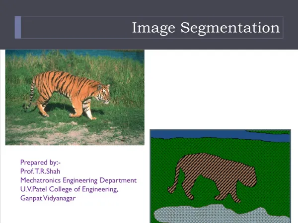
What is segmentation • Dividing an image to disjoint regions such that similar pixels are grouped together Image Courtesy: [3]
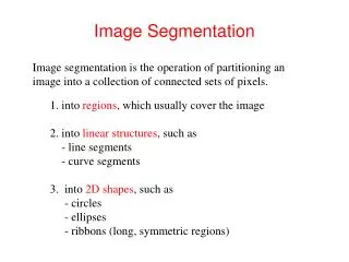
What is segmentation • Image Segmentation involves division of image I into K regions: R1, R2, R3, … RK such that: Every pixel must be assigned to a region Regions must be disjoint Size: 1 pixel to the entire image itself
What is segmentation • Pixels within a region share certain characteristics that is not found with pixels in another region. f is a function that returns TRUE if the region under consideration is homogenous
Applications of segmentation • Biomedical applications • Used as a preprocessing step to identify anatomical regions for medical diagnosis/analysis. Brain Tissue MRI Segmentation [1] CT Jaw segmentation [2]
Applications of segmentation • Object recognition systems: • Lower level features such as color and texture are used to segment the image • Only relevant segments (subset of pixels) are fed to the object recognition system. • Saves computational cost, especially for large scale recognition systems
Applications of segmentation • As a preprocessing step in face and iris recognition Face segmentation Iris Segmentation
Applications of segmentation • Astronomy: Preprocessing step before further analysis Segmentation of Nebula [4]
What is good segmentation? (Manual segmentations from BSDS) Which segmentation is “correct”?
What is good segmentation? • “Correctness”- Are similar pixels grouped together and dissimilar pixels grouped seperately? • Granularity- Extent of resolution of segmentation • Consider example in the previous image
What is good segmentation? • There is ambiguity in defining “good”/ “optimal” segmentation. • An image can have multiple segmentations. “correct” • Make evaluation /benchmarking of segmentation algorithm hard
Thesis overview • Related work • Background theory: • Image as a graph • Kruskals’ Minimum Spanning Tree • MST based segmentation • Our algorithm • Results • Conclusion and future work
Thesis overview • Related work • Background theory: • Image as a graph • Kruskals’ Minimum Spanning Tree • MST based segmentation • Our algorithm • Results • Conclusion and future work
Related work Some of the popular image segmentation approaches are: • Split and Merge approaches • Mean Shift and k-means • Spectral theory and normalized cuts • Minimum spanning tree
Related work • Split and Merge approaches • Iteratively split • If evidence of a boundary exists • Iteratively merge • Based on similarity • Quad-tree used Image Courtesy: [5]
Related work: Mean shift and k means • Mean shift and k-means are related. • Mean-shift: • Represent each pixel as a vector [color, texture, space] • Define a window around every point. • Update the point to the mean of all the points within the window. • Repeat until convergence.
Related work: Mean shift and k means • K-means: • Represent each pixel as vector [color, texture, space] • Choose K initial cluster centers • Assign every pixel to its closet cluster center. • Recompute the means of all the clusters • Repeat 1-2 until convergence. • Difference between K means and mean-shift: • In K-means, K has to be known beforehand • K-means sensitive to initial choice of cluster centers
Related work: Spectral theory and Normalized cuts • Represent image as a graph. • Using graph cuts, partitions the image into regions. • In Spectral theory and normalized cuts, • Eigenvalues/vectors of the Laplacian matrix is used to determine the cut
Related work: MST based approach • Use Minimum Spanning Tree to segment image. • Proposed by Felzenszwalb & Huttenlocher in 2004. • Uses a variant of Kruskals MST to segment images • Very efficient- O(NlogN) time • Discussed in detail in the next section
Thesis overview • Related work • Background theory: • Image as a graph • Kruskals’ Minimum Spanning Tree • MST based segmentation • Our algorithm • Results • Conclusion and future work
Background: Image as a graph • Graph G=(V,E) is an abstract data type containing a set of vertices V and edges E. • Useful operations using a graph: • See if path exists between any 2 vertices • Find connected components • Check for cycles • Find the shortest point between any 2 vertices • Compute minimum spanning • Graph partition based on cuts • Graph algorithms are useful in image processing
Background: Image as a graph • Image graph: • Pixels/group of pixels form vertices. • Vertices connected to form edges • Edge weight represents dissimilarity between vertices • Types of image graph: • Image grid • Complete graph • Nearest neighbor graph
Background: Image as a graph • Image grid: • Edges: every vertex (pixel) is connected with its 4 (or 8) x-y neighbors. • No of edges m= O(N) [Graph operations are quick] • Fails to capture global properties
Background: Image as a graph • Complete graph: • Edges: Connect every vertex (pixel) with every other vertex • No of edges m= O(N2) • Captures global properties • Graph operations are very expensive
Background: Image as a graph • Nearest neighbor graph: • Compromise between grid (fails to capture global properties) and complete graph (too many edges). • Represent every vertex as a combination of color and x-y features. [e.g. (R, G, B, x, y)] • Find the K=O(1) neighbors for each pixel using Approximate nearest neighbor (ANN) • Edges: Connect every pixel to K nearest neighbors
Thesis overview • Related work • Background theory: • Image as a graph • Kruskal’s Minimum Spanning Tree • MST based segmentation • Our algorithm • Results • Conclusion and future work
Background: Kruskal’s MST • Tree is a graph which is: • Connected • Has no cycles • Spanning tree: contains all the vertices of graph G • A graph can have multiple spanning trees • Minimum spanning tree is a spanning tree which has the least sum of weights of edges
Background: Kruskal’s MST • Sorting: O(mlog(m)) time • FindSet and Merge: O(mα(N)) time [very slow growing] • OVERALL TIME: O(m log(m))
Thesis overview • Related work • Background theory: • Image as a graph • Kruskal’s Minimum Spanning Tree • MST based segmentation • Our algorithm • Results • Conclusion and future work
Background: MST Segmentation • Use Minimum Spanning Tree to segment image. • In Kruskal’s MST algorithm, • Edges are sorted in ascending order of weights • Edges are added in order to the spanning tree as long as a cycle is not formed. • All vertices added to ONE spanning tree • If Kruskal’s is applied directly to image segmentation: • We will end up with ONE segment (entire image)
Background: MST Segmentation • Variant of Kruskal’s used in image segmentation. • Create an image grid graph. • Sort edges in the increasing order of weights • For every edge ei in E, • If FindSet(ui) ≠ FindSet(vi) AND IsSimilar(ui ,vi)=TRUE Merge(FindSet(ui) ,FindSet(vi) ) • Instead of one MST, we end up with a forest of K trees • Each tree represents a region
Background: MST Segmentation • We add an edge ei connecting regions Ru and Rv to a tree only if : • D(RuRv): edge weight connecting vertices u and v • Int(Ri): maximum edge weight in region Ri WE MERGE IF THE EDGE WEIGHT IS LOWER THAN THE MAXIMUM EDGE WEIGHT IN EITHER REGIONS!!
Background: MST Segmentation • Drawback 1: LEAK Felzenszwalb and Huttenlocher 2004
Background: MST Segmentation • Drawback 2: SENSITIVITY TO PARAMETER k • Notice how granularity changes by varying k • k is arbitrary • k is affected by the size of the image
Thesis overview • Related work • Background theory: • Image as a graph • Kruskal’s Minimum Spanning Tree • MST based segmentation • Our algorithm • Results • Conclusion and future work
Our algorithm: overview • Objective • Constructing image grid • Sort edges in ascending order • For every edge • If Merge criterion is satisfied • Merge
Our algorithm: Objective • Improve upon the drawbacks of MST ALGORITHM: • Addressing Leak: • Represent regions as a Gaussian distribution. • Use Bidirectional Mahalanobis distance to compare Gaussians. • Overcome sensitivity to parameter k: • Propose parameter τ that is • independent of image size • Works well for 2-2.5 • Provide a mathematical intuition for it. • Propose an approximation that enables real-time implementation.
How to compare two regions in a graph?MST APPROACH Int(Ru) Int(Rv) D(u,v) u v • Check if D(u,v) < Int(Ru) && D(u,v) < Int(Rv) • Leak can happen
How to compare two regions in a graph?OUR APPROACH D(u,v) u v • Represent each region as a Gaussian • Check if the Gaussians are similar: • Mahalanobis distance is less than 2.5
Our algorithm: overview • Objective • Constructing image grid • Sort edges in ascending order • For every edge • If Merge criterion is satisfied • Merge
Our algorithm: Building image grid • Initialize Vertices: • Every pixel is mapped to a vertex • Information about vertex vi is stored at the ‘i’th entry of the disjoint set data structure D. • The ‘i’th entry in D contains following information: • Root node • Zeroth, first and second order moments • List of all the edges connected to vertex vi
Our algorithm: Building image grid • Initialize Edges: • Between neighboring pixels in x-y space • Number of edges m= O(N) • Use List to maintain edges • Edge weight: • Euclidean distance between pixels to begin with • Mahalanobis distance between Gaussians as region grows • Note that Euclidean distance is a special instance of Mahalanobis distance
Our algorithm: overview • Objective • Constructing image grid • Sort edges in ascending order • For every edge • If Merge criterion is satisfied • Merge
Our algorithm: overview • Objective • Constructing image grid • Sort edges in ascending order • For every edge • If Merge criterion is satisfied • Merge
Our algorithm: Merge Criterion • While adding edge ei to the MST, regions Ru and Rv are merged if the following criterion is satisfied: Forces small regions to merge Around 2.5 is a good threshold Bidirectional Mahalanobis
Our algorithm: overview • Objective • Constructing image grid • Sort edges in ascending order • For every edge • If Merge criterion is satisfied • Merge
Our algorithm: Merge • Merging regions Ru and Rv • Update information at the root node of the disjoint set data-structure (Similar to MST) • Updating information about root node, zeroth, first and second order moment is easy • However, after merging Ru and Rv • All edges connected to either Ru or Rvhave to be updated w.r.t. (Ru ∪ Rv) • The edges have to be re-sorted. • The above operations will slow down the overall running time to O(N2).
Our algorithm: Speed-up • To speed up weight update that needs to be performed after every iteration, • For every region in the DSDS, we store the pointers to all the edges connected to it. • When 2 regions are merged, we merge their neighbor lists also • Assuming that the number of neighbors for every region is constant, every iteration of merging neighbors can also be accomplished in O(1) time

