Download
1 / 40
400 likes | 812 Vues
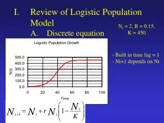
I. Review of Logistic Population Model. N t = 2, R = 0.15, K = 450. A. Discrete equation. - Built in time lag = 1 - Nt+1 depends on Nt. I. Review of Logistic Population Model. B. Density Dependence. Review of Logistic Population Model C. Assumptions.

E N D
I. Review of Logistic Population Model Nt = 2, R = 0.15, K = 450 A. Discrete equation - Built in time lag = 1 - Nt+1 depends on Nt
I. Review of Logistic Population Model B. Density Dependence
Review of Logistic Population ModelC. Assumptions • No immigration or emigration • No age or stage structure to influence births and deaths • No genetic structure to influence births and deaths • No time lags in continuous model
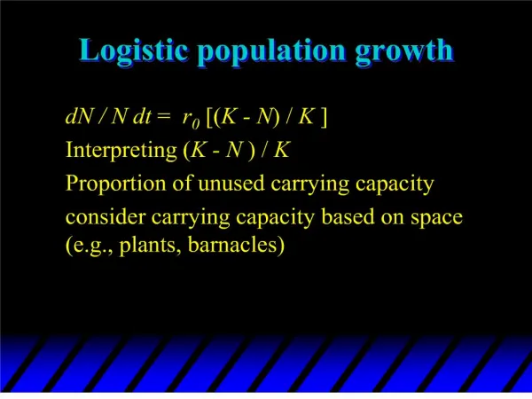
K Review of Logistic Population ModelC. Assumptions • Linear relationship of per capita growth rate and population size (linear DD)
Review of Logistic Population ModelC. Assumptions • Linear relationship of per capita growth rate and population size (linear DD) • Constant carrying capacity – availability of resources is constant in time and space • Reality?
I. Review of Logistic Population Model Discrete equation Nt = 2, r = 1.9, K = 450 Damped Oscillations r <2.0
I. Review of Logistic Population Model Discrete equation Nt = 2, r = 2.5, K = 450 Stable Limit Cycles 2.0 < r < 2.57 * K = midpoint
I. Review of Logistic Population Model Discrete equation Nt = 2, r = 2.9, K = 450 • Chaos • r > 2.57 • Not random • change • Due to DD • feedback and time • lag in model
Review of Logistic Population ModelD. Deterministic vs. Stochastic Models Nt = 1, r = 2, K = 100 * Parameters set deterministic behavior same
Nt = 1, r = 0.15, SD = 0.1; K = 100, SD = 20 Review of Logistic Population ModelD. Deterministic vs. Stochastic Models * Stochastic model, r and K change at random each time step
Nt = 1, r = 0.15, SD = 0.1; K = 100, SD = 20 Review of Logistic Population ModelD. Deterministic vs. Stochastic Models * Stochastic model
Nt = 1, r = 0.15, SD = 0.1; K = 100, SD = 20 Review of Logistic Population ModelD. Deterministic vs. Stochastic Models * Stochastic model
Environmental StochasticityA. Defined • Unpredictable change in environment occurring in time & space • Random “good” or “bad” years in terms of changes in r and/or K • Random variation in environmental conditions in separate populations • Catastrophes = extreme form of environmental variation such as floods, fires, droughts • High variability can lead to dramatic fluctuations in populations, perhaps leading to extinction
Environmental StochasticityA. Defined • Unpredictable change in environment occurring in time & space • Random “good” or “bad” years in terms of changes in r and/or K • Random variation in environmental conditions in separate populations • Catastrophes = extreme form of environmental variation such as floods, fires, droughts • High variability can lead to dramatic fluctuations in populations, perhaps leading to extinction
Environmental StochasticityA. Defined • Unpredictable change in environment occurring in time & space • Random “good” or “bad” years in terms of changes in r and/or K • Random variation in environmental conditions in separate populations • Catastrophes = extreme form of environmental variation such as floods, fires, droughts • High variability can lead to dramatic fluctuations in populations, perhaps leading to extinction
Environmental StochasiticityB. Examples – variable fecundity Relation Dec-Apr rainfall and number of juvenile California quail per adult (Botsford et al. 1988 in Akcakaya et al. 1999)
Environmental StochasiticityB. Examples - variable survivorship Relation total rainfall pre-nesting and proportion of Scrub Jay nests to fledge (Woolfenden and Fitzpatrik 1984 in Akcakaya et al. 1999)
Environmental StochasiticityB. Examples – variable rate of increase Muskox population on Nunivak Island, 1947-1964 (Akcakaya et al. 1999)
Environmental StochasiticityC. Incorporating into Logistic Model Random variable with mean and variance
II. Environmental StochasiticityC. Incorporating into Logistic Model • Randomize r and/or K for each time step • Using Excel, =NORMINV(RAND( ), mean, sd) function provides random variable based on normal distribution with specified mean & variance
Nt = 2, r = 0.15, SD = 0.1; K = 100 Environmental StochasiticityC. Incorporating into Logistic Model • Random r, K is constant * Stochastic model behavior
Nt = 2, r = 0.15, SD = 0.1; K = 100 Environmental StochasiticityC. Incorporating into Logistic Model • Random r, K is constant
Nt = 2, r = 0.15, SD = 0.1; K = 100 Environmental StochasiticityC. Incorporating into Logistic Model • Random r, K is constant
Environmental StochasiticityC. Incorporating into Logistic Model • Random r, K is constant General Trend: • Population grows erratically at smaller population sizes, stabilizes close to K
Nt = 2, r = 0.15; K = 100, SD = 20 Environmental StochasiticityC. Incorporating into Logistic Model • Constant r, K is random
Nt = 2, r = 0.15; K = 100, SD = 20 Environmental StochasiticityC. Incorporating into Logistic Model • Constant r, K is random
Nt = 2, r = 0.15; K = 100, SD = 20 Environmental StochasiticityC. Incorporating into Logistic Model • Constant r, K is random
Environmental StochasiticityC. Incorporating into Logistic Model • Constant r, K is random General Trend: • Variation observed mainly at or near K
Environmental Stochasiticity- Example of random K • Serengeti wildebeest data set – recovering from Rinderpest outbreak • Fluctuations around K possibly related to rainfall
Environmental StochasiticityC. Incorporating into Logistic Model • Constant r, K is random • Mean N always less than mean K • Population rate of change differs above or below K
Environmental StochasiticityC. Incorporating into Logistic Model • Constant r, K is random • More variable environment = smaller average population size
Large r = track changes in K, N = close to K • Small r = slower to track changes in K • Random K, influence of r on population fluctuations R = 0.1 R = 0.8
Nt = 2, r = 0.15; SD = 0.1; K = 100, SD = 20 Environmental StochasiticityC. Incorporating into Logistic Model • Random r & K
Nt = 2, r = 0.15; SD = 0.1; K = 100, SD = 20 Environmental StochasiticityC. Incorporating into Logistic Model • Random r & K
Nt = 2, r = 0.15; SD = 0.1; K = 100, SD = 20 Environmental StochasiticityC. Incorporating into Logistic Model • Random r & K
Environmental StochasiticityC. Incorporating into Logistic Model • Random r & K General Trend: • Variation observed throughout population sizes
Environmental StochasiticityE. Implications & Caveats • Application of principle to Population Viability Analysis (PVA) & population forecasting
Environmental StochasiticityE. Implications & Caveats • Sampling variation & parameter uncertainty • All measurements have error…parameter uncertainty = variation in estimate of parameter due to accuracy & precision of sampling protocol • must account for portion of variation in estimates of vital rates determined by sampling (i.e., separate from “natural” sources of variation)