logistic population growth
Filling carrying capacity. Filling carrying capacity. Filling carrying capacity. Filling carrying capacity. Logistic growth: Numerical Example (let r0 = 0.10, K = 100). Logistic growth: Numerical Example (let r = 0.10, K = 100). . Nt. dN /Ndt. K=100. K / 2=50. r0 = 0.10. 0. Logistic growth: Numerical Example (let r0 = 0.10, K = 100).

logistic population growth
E N D
Presentation Transcript
1. Logistic population growth dN / N dt = r0 [(K - N) / K ]
Interpreting (K - N ) / K
Proportion of unused carrying capacity
consider carrying capacity based on space (e.g., plants, barnacles)
2. Filling carrying capacity
3. Filling carrying capacity
4. Filling carrying capacity
5. Filling carrying capacity
6. Logistic growth: Numerical Example(let r0 = 0.10, K = 100)
7. Logistic growth: Numerical Example(let r = 0.10, K = 100)
8. Logistic growth: Numerical Example(let r0 = 0.10, K = 100)
9. Logistic population decline
10. Assumptions of logistic growth model K is constant over time
does not vary year to year etc.
dN / Ndt declines linearly with N
alternative � nonlinear decline
Effect of density N on dN / Ndt is instantaneous � no delays
alternative � density now affects dN / Ndt some time in the future (time lag)
Continuous overlapping generations
11. Logistic growth: Real data
12. Discrete Logistic: non-overlapping generations e.g., Seasonal reproduction
Difference equation model
DN = Nt+1 - Nt = r0 Nt [ (K - Nt ) / K ]
Note: this notation is different from that in Krebs (pp. 158-159)
See Gotelli Ch. 2, pp. 37-39
Unlike continuous logistic, many odd and complex dynamics result
Note: not necessarily semelparous
13. Discrete Logistic Outcomes r0 < 2.0 � Damped Oscillations
14. Discrete Logistic Outcomes2.00 < r0 < 2.45 � Stable 2-point cycle
15. End 19th lecture
16. Discrete Logistic Outcomes 2.45 < r0 < 2.50 �more complex cycles
17. Discrete Logistic Outcomes 2.50 < r0 < 2.57 �more complex cycles
18. Discrete Logistic Outcomes r0 > 2.57 � Chaos
19. Cycles & chaos in discrete logistic low r0 (<2.0) � very simple dynamics
as r0 increases � 2, 4, 8, 16, 32 , etc. point cycles
r0 > 2.57 � deterministic chaos
non-repeated oscillations
slightly different starting conditions yield completely different dynamics
20. Discrete Logistic Outcomes Chaos � dynamics depend on initial conditions
21. Importance of cycles and chaos Annual, discrete generations common
Insects (and others) frequently go through cycles and complex fluctuations in nature
Traditional interpretation � annual random variation in conditions
Cycles and chaos may be products of the deterministic dynamics, not variation
22. aphid -- 2 point cycle
aphid -- chaos
moth -- damped
moth -- damped
moth -- damped
yellow jacket -- damped
23. Denisty dependent population growth Logistic growth implies density dependence
Population is Regulated
Density dependence is what stops population increase
Density independent effects also implact logistic populations
Population Limitation
24. Density independent effects Logistic population growth
Density dependent b
Density independent d
e.g. due to weather
If density independent d differs, K will differ
But b is what regulates population
25. Harvesting We harvest natural populations
How much can be harvested in any year?
Is the population to remain stable?
�Stock� = harvestable part of population
Stock:
decreases due to mortality and harvest
increases due to growth and recruitment
�recruitment� = fish attain catchable size
26. Harvesting S2 = S1 + R + G � M � F
Where:
S1 = Stock at start of year
S2 = Stock at end of year
R = Recruits
G = Growth
M = Natural mortality
F = Fishing yield
27. Harvesting
28. Exam #2
29. Continuous vs. Discrete generations