Spatial Dimensions of Environmental Regulations

1. Spatial Dimensions of Environmental Regulations What happens to simple regulations when space matters? Hotspots? Locational differences?

2. Motivation • Group Project on Newport Bay TMDL • What rules on maximum emissions from different industries will assure acceptable level of water quality in Newport Bay? • Reference: http://www.bren.ucsb.edu/research/2002Group_Projects/Newport/newport_final.pdf

3. Example: Carpinteria marsh problem • Many creeks flow into Carpinteria salt marsh; pollution sources throughout. • Pollution mostly in form of excess nutrients (e.g. Nitrogen & Phosphorous) • How should pollution be controlled at each upstream source to achieve an ambient standard downstream?

4. Carpinteria Salt Marsh

5. Salt Marsh

6. The Carpinteria Marsh problem x x x x x x x x Marsh o Where we care about pollution: receptor (o) Where pollution originates: sources (x)

7. Sources and Receptors • Sources are where the pollutants are generated – index by i. [“emissions”] • Receptors are where the pollution ends up and where we care about pollution levels – index by j. [“pollution”] • Emissions: e1, e2, …, eI (for I sources) • Pollution concentrations: p1, p2,…,pJ • Connection: pj=fj(e1,e2,…,eI) • “Transfer function”—from Arturo

8. “Transfer coefficients” • Typically f is linear (makes life simple) • pj = Saijei + Bj • Where B is the background level of pollution • aij is “transfer coefficient” • dfj/dei= aij = transfer coefficient (if linear) • Interpretation of aij: if emissions increase in a greenhouse on Franklin Creek, how much does concentration change in salt marsh? • What causes the aij to vary? • Distance, natural attenuation and dispersion • Higher transfer coefficient = higher impact of source on receptor

9. Example: concrete-lined channelDoes this increase or decrease transfer coefficient?

10. Add some economics: Simple case of one receptor • Emission control costs depend on abatement: • Ai = Ei – ei where • Ei = uncontrolled emissions level (given) • ei = controlled level of emissions (a variable) • E.g. ci(Ai) = ai + bi(Ai) + gi(Ai)2 • Control costs (by industry) often available from EPA, other sources (e.g. Midterm) • What is marginal cost of abatement? • MCi(Ai) = βi +2 gi Ai

11. How much abatement? • To achieve ambient standard, S, which sources should abate and how much? • Problem of finding least cost way of achieving S MineSi ci(Ei-ei) s.t. Si aiei≤ S • In words: minimize abatement cost such that total pollution at Carpinteria Salt Marsh ≤ S.

12. Solution (mathematical) • Set up Lagrangian • L = Σici(Ei-ei) + µ (Saiei- S) • Differentiate with respect to ei, µ • ∂L/∂ei = -MCi(Ei-ei) + µ ai = 0 for all i •  equalize MCi/ai = µ for all i • Solution: find ei such that • Marginal abatement cost normalized by transfer coefficient is equal for all sources (interpretation?) • Resulting pollution level is just equal to standard

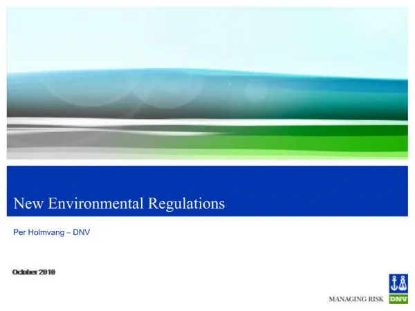
13. Spatial equi-marginal principle • Instead of equating marginal costs of all polluters, need to adjust for different contributions to the receptor. • All sources are controlled so that marginal cost of emissions control, adjusted for impact on the ambient, is equalized across all sources. • MCi / ai equal for all sources. • Sources with big “a”’s controlled more tightly

14. Effect of higher “a” MCA(a low) MCA(a high) MCB MCA Abatement

15. What kind of regulations would achieve desired level of pollution? • Rollback • Standard engineering solution. • Desired pollution level x% of current level  reduce all sources by x% • Marketable permits – no spatial differentiation • Polluters with big transfer coefficients would not control enough • Polluters with small transfer coefficients would control too much. • Constant fee to all polluters • Same problem as permits

16. Spatial Version of Marketable Permits • Issue 10 permits to degrade Salt Marsh • Allowed emissions for source i, holding x permits: ei=xi/ai. • What is total pollution at receptor? • Saiei= Sai(xi/ai) = Sxi = 10 • Does the equimarginal principle hold? • Price of permit = π (cost for i: π xi) • Price per unit emissions = π xi/ ei= π xi /(xi/ai) = π ai • For each source, marginal cost divided by ai = π • Therefore, Equimarginal Principle Holds • Idea: Trade or value damages not emissions.

17. Constructing a Policy Analysis ModelCarpinteria Salt Marsh Example • Variables of interest • i=1,…,I sources • ei, emissions by source i • Ai, pollution abatement by source i • Data needed • Ci(Ai), pollution control cost function for source i • Ei, uncontrolled emissions by source i • ai, transfer coefficient for source i • S, upper limit on pollution at single receptor

18. Model Construction • Goal is to minimize cost of meeting pollution concentration objective • Objective function (minimize): • Σici(Ai) = Σi [ai + bi(Ai) + gi(Ai)2] or • Σici(Ei-ei) = Σi [ai + bi(Ei-ei) + gi(Ei-ei)2] • Constraints • Si aiei≤ S • ei ≥ 0 (non-negativity constraint) • Solve using Excel or other optimization software

19. Policy Experiments with Model • What is the least cost way of meeting S? • Always start with this baseline • Can be achieved through spatially differentiated permits • Consider a variety of different policies • Rollback • Simple (non-spatially differentiated) emission permits

20. Policy Experiments with Model: Rollback • How much would it cost to achieve S using rollback? • Calculate pollution from current emissions, Ei • Calculate percent rollback and then emissions • Compute costs of this emission level

21. Policy Experiments with ModelEmission permits • Why? • Simpler than spatially differentiated emission permits • How much would it cost to use emission permits (non-spatially differentiated)? • Eliminate constraint on pollution and substitute Si ei≤ E+ where E+ is number of permits issued • This simulates how a market for E+ emission permits would operate • Calculate resulting pollution levels: Si aiei = S+ • How do you think the cost of achieving S+ with emission permits will compare to the least cost way of achieving S+? • Vary E+, until S+ exactly equals S. • Bingo! You know the amount of emission permits to issue

22. What might the results look like? Rollback Approach Emission Permits Least Cost Total Pollution Control Costs ($) Uncontrolled pollution levels at Marsh 0 Pollution at Salt Marsh Note: order of costs need not be as shown.