Bijective tree encoding
Bijective tree encoding. Saverio Caminiti. Talk Outline. Domains Prüfer-like codes Prüfer code (1918) Neville codes (1953) Deo and Micikevičius code (2002) Picciotto codes (1999) Applications, Operations and Properties Random trees generation (with constrains) Locality and Heritability

Bijective tree encoding
E N D
Presentation Transcript
Bijective tree encoding Saverio Caminiti
Talk Outline • Domains • Prüfer-like codes • Prüfer code (1918) • Neville codes (1953) • Deo and Micikevičius code (2002) • Picciotto codes (1999) • Applications, Operations and Properties • Random trees generation (with constrains) • Locality and Heritability • Other operations • Future work
Domains • Labeled trees Tn • n nodes labeled with distinct symbols in s.t. || = n i.e. indexed with integers in [n] = {1, 2, ..., n} • Both rooted and unrooted • Undirected • No ordered among nodes children • Strings according with Cayley’s theorem • In n-2 for unrooted (i.e. [n]n-2) • In n-1 for rooted (i.e. [n]n-1)
1 3 6 4 5 4 2 1 3 6 2 5 Examples 4 1 3 3 1 4 3 3 4
Prüfer code • Introduced in 1918 to prove the Cayley’s theorem is the first bijection between Tn and [n]n-2 (T) = adj(u) :: (T-u) • where: • u is the smallest leaf in T, • adj(u) is the only node adjacent to u in T, • T-u is the tree obtained from T removing u, • and the operator :: is the string concatenation.
Example: Prüfer encode unrooted (T) = adj(u) :: (T-u) • S 2 4 1 5 3 • C 4 1 3 3 6 1 3 6 = n 4 5 2 = n n - 2
Example: Prüfer encode rooted (T) = adj(u) :: (T-u) • S 2 1 5 6 3 • C 1 4 3 3 4 4 = n 1 3 6 2 5 = n n - 1
Notes: Prüfer encode (T) = adj(u) :: (T-u) • S 2 1 5 6 3 • C 1 4 3 3 4 Focus on rooted trees • Each node (but the root) is removed exactly once • Each node appear in C once for each children • A node can be removed only after all its children 4 1 3 6 2 5 n - 1
Example: Prüfer decode • C 1 4 3 3 4 • S ? ? ? ? ? • Let l be the length of the string C • n = l + 1 = 6 • First step: the leaves of initial tree are those nodes that do not appear in C: {2, 5, 6} choose the smallest one
Example: Prüfer decode • C 1 4 3 3 4 • S 2 • The remaining code 4 3 3 4 is (T-{2})then we should choose the smallest leaf among {1, 5, 6}
Example: Prüfer decode • C 1 4 3 3 4 • S 2 1 • The remaining code 3 3 4 is (T-{2, 1})then we should choose the smallest leaf among {5, 6}
4 1 3 6 2 5 Example: Prüfer decode • C 1 4 3 3 4 • S 2 1 5 6 3
Other Prüfer-like codes • Neville (1953) for rooted trees • The first one was indeed the Prüfer code • Moon (1970) • Adapts Neville’s codes to trees • Deo and Micikevičius (2002)
Generalization • It has been proven that any deterministic procedure P able to choose at each stepa non- empty sequence of leaves can be usedto generate a bijective code (T) = adj(P(T)) :: (T-P(T))
Why several codes • Different codes may have different properties and allow different operations • Encoding and Decoding algorithms for different code may have different time (and/or space) complexity
Implementation of Prüfer code • Straightforward implementation: O(n log n) • First linear time algorithm in 1978(left as exercise in Combinatorial algorithms) • Optimal parallel algorithm 2000 • Linear time sequential algorithm rediscovered in 2000 and 2001 • Still unknown in 2003 !!!
Implementation of other codes • Second Neville code 2002 • Third Neville code 1953 (trivial) • Deo and Micikevičius 2002(in the original paper)
A unified approach • The encoding of all four codes can be reduce to sorting pairs integer in [n] • The decoding can be reduced to the computation of the rightmost occurrence of each symbol in the code string
Encoding: Second Neville code • pair 0,3 0,4 0,5 0,8 0,9 1,1 1,6 1,10 2,2 • S 3 4 5 8 9 1 6 10 2 • C 6 10 6 1 7 2 7 7 7 (l(v), v) where l(v) is the level of v from the bottom
Encoding: Third Neville code • pair 3,0 4,0 4,1 5,0 5,1 8,0 8,1 8,2 8,3 • S 3 4 10 5 6 8 1 2 7 • C 6 10 7 6 7 1 2 7 9 ( (v), d(v, (v)) ) where (v) is the greatest leaf in the subtree rooted at v
Linear time implementation • All the information appearing in pairs can be computer with a simple tree traversal O(n) • To sort the set of pairs it is enough to execute twice a stable integer sort O(n)
Decoding: Third Neville code • C 6 10 7 6 7 1 2 7 9 • S ? ? ? ? ? ? ? ? ? • Compute the rightmost occurrence of eachv [n] into C: v 1 2 3 4 5 6 7 8 9 10 v 6 7 0 0 0 4 8 0 9 2
Decoding: Third Neville code • C 6 10 7 6 7 1 2 7 9 • S ? ? ? ? ? ? ? ? ? • Compute the rightmost occurrence of eachv [n] into C: v 1 2 3 4 5 6 7 8 9 10 v 6 7 0 0 0 4 8 0 9 2
Decoding: Third Neville code • C 6 10 7 6 7 1 2 7 9 • S ? ? 10 ? 6 ? 1 2 7 • Compute the rightmost occurrence of eachv [n] into C: v 1 2 3 4 5 6 7 8 9 10 v 6 7 0 0 0 4 8 0 9 2
Decoding: Third Neville code • C 6 10 7 6 7 1 2 7 9 • S 3 4 10 5 6 8 1 2 7
Parallel results • These techniques allow us to efficiently encode and decode on EREW PRAM: • Integer Sorting require O(log n) timeand O(n √ log n) operations • The rightmost occurrence computation can be reduced to Integer Sorting
Talk Outline • Domains • Prüfer-like codes • Prüfer code (1918) • Neville codes (1953) • Deo and Micikevičius code (2002) • Picciotto codes (1999) • Applications, Operations and Properties • Random trees generation (with constrains) • Locality and Heritability • Other operations • Future work
Picciotto’s codes • In her PhD thesis Picciotto proposed three codes for unrooted trees: • Blob code • Happy code • Dandelion code • Easily adapted to rooted tree (T, r) c1 c2 ... cn-2r n - 1
Happy code 0 6 2 3 5 4 7 1
Happy code 0 6 2 3 5 4 7 1
Happy code 0 6 3 2 5 4 7 1
Happy code 0 3 2 6 4 5 7 1
Happy code 0 3 2 6 4 5 7 1 Node 2 3 4 5 6 7 C 0 4 3 6 6 5
Happy code x f(x) 0 0 1 0 2 0 3 4 4 3 5 6 6 6 7 7 0 3 2 6 4 5 7 1 Node 2 3 4 5 6 7 C 0 4 3 6 6 5
Happy code • Create a bijection between Tn and a subset of the endofunctions on [n] {ƒ:[n][n] s.t. ƒ(0) = ƒ(1) = 0} • The code string is ƒ(2) :: ƒ(3) :: ... :: ƒ(n) • Linear time encoding and decoding(identify and break cycles, reconstruct the original path from 1 to 0)
Blob code 0 5 2 3 1 4 Node 1 2 3 4 5 C
Blob code 0 5 2 3 1 4 Node 1 2 3 4 5 C -
Blob code 0 5 2 3 1 4 Node 1 2 3 4 5 C 0 -
Blob code path(3, 0) Blob 3 is stable 0 5 2 3 1 4 Node 1 2 3 4 5 C 5 0 -
Blob code 0 5 2 3 1 4 Node 1 2 3 4 5 C 2 5 0 -
Blob code path(1, 0) Blob 1 is stable 0 5 2 3 1 4 Node 1 2 3 4 5 C 2 2 5 0 -
Blob code • Straight forward implementation leads to O(n2)(used in 2003) • Can be reduced to the transformation of the tree in a functional digraph • Linear time encoding and decoding algorithm
Blob code path(v, 0) contains u > vv is stable 0 5 2 3 1 4 Node 1 2 3 4 5 C 2 5 -
Blob code 0 5 2 3 1 4 Node 1 2 3 4 5 C 2 2 5 0 -
Blob code x f(x) 0 0 1 2 2 2 3 5 4 0 5 0 0 5 2 3 1 4 Node 1 2 3 4 5 C 2 2 5 0 - ƒ(1) ƒ(2) ƒ(3) ƒ(4)
Dandelion code Node 2 3 4 5 6 7 8 9 10 11 C 5 6 10 2 4 2 1 0 3 9
Dandelion code Node 2 3 4 5 6 7 8 9 10 11 C 5 6 10 2 4 2 1 0 3 9