Measurement System Behavior
2141-375 Measurement and Instrumentation. Measurement System Behavior. Dynamic Characteristics.

Measurement System Behavior
E N D
Presentation Transcript
2141-375 Measurement and Instrumentation Measurement System Behavior
Dynamic Characteristics Dynamic characteristics tell us about how well a sensor responds to changes in its input. For dynamic signals, the sensor or the measurement system must be able to respond fast enough to keep up with the input signals. Sensor or system Output signal y(t) Input signal x(t) In many situations, we must use y(t) to infer x(t), therefore a qualitative understanding of the operation that the sensor or measurement system performs is imperative to understanding the input signal correctly.
y(0) x(t) y(t) Measurement system General Model For A Measurement System nth Order ordinary linear differential equation with constant coefficient F(t) = forcing function Where m ≤ n y(t) = output from the system x(t)= input to the system t = time a’s andb’s= system physical parameters, assumed constant The solution Whereyocf = complementary-function part of solution yopi= particular-integral part of solution
Complementary-Function Solution The solutionyocf is obtained by calculating the n roots of the algebraic characteristic equation Characteristic equation Roots of the characteristic equation: Complementary-function solution: 1. Real roots, unrepeated: 2. Real roots, repeated: each root s which appear p times 3. Complex roots, unrepeated: the complex form: a ib 4. Complex roots, repeated: each pair of complex root which appear p times
Particular Solution Method of undetermined coefficients: Where f(t) = the function that describes input quantity A, B, C = constant which can be found by substitutingyopiinto ODEs Important Notes • After a certain-order derivative, all higher derivatives are zero. • After a certain-order derivative, all higher derivatives have the same functional form as some lower-order derivatives. • Upon repeated differentiation, new functional forms continue to arise.
Zero-order Systems All the a’s and b’s other than a0 and b0 are zero. whereK = static sensitivity = b0/a0 The behavior is characterized by its static sensitivity, K and remains constant regardless of input frequency (ideal dynamic characteristic). xm Vr + Where 0 x xmandVris a reference voltage y = V x = 0 - A linear potentiometer used as position sensor is a zero-order sensor.
First-Order Systems All the a’s and b’s other than a1, a0 and b0 are zero. WhereK = b0/a0is the static sensitivity = a1/a0 is the system’s time constant(dimension of time)
First-Order Systems: Step Response Assume for t < 0, y = y0 , at time = 0 the input quantity, x increases instantly by an amount A. Therefore t > 0 The complete solution: yopi yocf Transient response Steady state response Applying the initial condition, we get C = y0-KA, thus gives
First-Order Systems: Step Response Here, we define the term error fraction as Non-dimensional step response of first-order instrument
Determination of Time constant 0.368 Slope = -1/
Assume that at initial condition, both y and x = 0, at time = 0, the input quantity start to change at a constant rate Thus, we have First-Order Systems: Ramp Response Therefore The complete solution: Steady state response Transient response Applying the initial condition, gives Measurement error Steady state error Transient error
First-Order Instrument: Ramp Response Steady state time lag= Steady state error= Non-dimensional ramp response of first-order instrument
First-Order Systems: Frequency Response From the response of first-order system to sinusoidal inputs, we have The complete solution: Transient response Steady state response Frequency response = If we do interest in only steady state response of the system, we can write the equation in general form Where B() = amplitude of the steady state response and () = phase shift
First-Order Instrument: Frequency Response The amplitude ratio The phase angle is Dynamic error -3 dB 0.707 Cutoff frequency Frequency response of the first order system Dynamic error, () = M(): a measure of an inability of a system to adequately reconstruct the amplitude of the input for a particular frequency
Dynamic Characteristics Frequency Response describe how the ratio of output and input changes with the input frequency. (sinusoidal input) Dynamic error, () = 1- M()a measure of the inability of a system or sensor to adequately reconstruct the amplitude of the input for a particular frequency Bandwidththe frequency band over which M() 0.707 (-3 dB in decibel unit) Cutoff frequency:thefrequency at which the system response has fallen to 0.707 (-3 dB) of the stable low frequency.
First-Order Systems: Frequency Response Ex: Inadequate frequency response Suppose we want to measure x(t) With a first-order instrument whose is 0.2 s and static sensitivity K Superposition concept: For = 2 rad/s: y(t)/K For = 20 rad/s: Therefore, we can write y(t) as
Dynamic Characteristics Example:A first order instrument is to measure signals with frequency content up to 100 Hz with an inaccuracy of 5%. What is the maximum allowable time constant? What will be the phase shift at 50 and 100 Hz? Solution: Define From the condition |Dynamic error| < 5%, it implies that But for the first order system, the term can not be greater than 1 so that the constrain becomes Solve this inequality give the range The largest allowable time constant for the input frequency 100 Hz is The phase shift at 50 and 100 Hz can be found from This give = -9.33oand = -18.19oat 50 and 100 Hz respectively
Second-Order Systems In general, a second-order measurement system subjected to arbitrary input, x(t) The essential parameters = the static sensitivity = the damping ratio, dimensionless = the natural angular frequency
Second-Order Systems Consider the characteristic equation This quadratic equation has two roots: Depending on the value of , three forms of complementary solutions are possible Overdamped ( > 1): Critically damped ( = 1): Underdamped (< 1)::
Second-Order Systems Case I Underdamped (< 1): Case 2 Overdamped ( > 1): Case 3Critically damped ( = 1):
Second-order Systems Example: The force-measuring spring consider a spring with spring constant Ks under applied force fi and the total mass M. At start, the scale is adjusted so that xo= 0 when fi = 0; the second-order model:
Second-order Systems: Step Response For a step input x(t) With the initial conditions: y = 0 at t = 0+, dy/dt = 0 at t = 0+ The complete solution: Overdamped ( > 1): Critically damped ( = 1): Underdamped (< 1)::
Second-order Instrument: Step Response Ringing frequency: Ringing frequency: = 0 0.25 Rise time decreases with but increases ringing 0.5 Optimum settling time can be obtained from ~ 0.7 1.0 Practical systems use 0.6< <0.8 2.0 Non-dimensional step response of second-order instrument
Dynamic Characteristics overshoot 100% 5% settling time rise time Typical response of the 2nd order system
Second-order System: Ramp Response For a ramp input With the initial conditions: y = dy/dt = 0 at t = 0+ The possible solutions: Overdamped: Critically damped: Underdamped:
Second-order Instrument: Step Response Steady state error = Steady state time lag= Ramp input = 0.3 0.6 1.0 2.0 Typical ramp response of second-order instrument
Second-order Instrument: Frequency Response The response of a second-order to a sinusoidal input of the form x(t) = Asint where The steady state response of a second-order to a sinusoidal input Where B() = amplitude of the steady state response and () = phase shift
0 = 0.1 0.3 = 0.1 0.5 0.3 1.0 0.5 2.0 1.0 2.0 Second-order Instrument: Frequency Response The phase angle The amplitude ratio Magnitude and Phase plot of second-order Instrument
Second-order Systems For overdamped ( >1) or critical damped ( = 1), there is neither overshoot nor steady-state dynamic error in the response. In an underdameped system ( < 1) the steady-state dynamic error is zero, but the speed and overshoot in the transient are related. Td overshoot Rise time: Maximum overshoot: Peak time: peak time Resonance frequency: settling time Resonance amplitude: rise time
Dynamic Characteristics Speed of response: indicates how fast the sensor (measurement system) reacts to changes in the input variable. (Step input) Rise time: the length of time it takes the output to reach 10 to 90% of full response when a step is applied to the input Time constant: (1st order system) the time for the output to change by 63.2% of its maximum possible change. Settling time: the time it takes from the application of the input step until the output has settled within a specific band of the final value. Dead time: the length of time from the application of a step change at the input of the sensor until the output begins to change