Download
1 / 29
360 likes | 885 Vues
Basics of Spectroscopy. Gordon Robertson (University of Sydney). Outline. Aims of spectroscopy Variety of instrumentation - formatting to a 2D detector Diffraction gratings Optical setups, Grating equation, Spectral resolution Prisms Volume Phase Holographic gratings The A product

E N D
Basics of Spectroscopy Gordon Robertson (University of Sydney)
Outline • Aims of spectroscopy • Variety of instrumentation - formatting to a 2D detector • Diffraction gratings • Optical setups, Grating equation, Spectral resolution • Prisms • Volume Phase Holographic gratings • The A product • Conclusion
Science goals of spectroscopy 1. Elemental composition and abundances 2. Kinematics 3. Redshifts / cosmology i.e. what is it, where is it, what are its internal motions…. For stars, star clusters, nebulae, galaxies, AGN, intervening clouds etc...
Aims of spectroscopic observations Ideally…. A data cube, covering a wide range in each of ,, With good …. spatial resolution , , wavelength resolution , and efficiency BUT detectors are 2-dimensional, so the data must be formatted to fit them. Many interesting new ways of dealing with this.
Narrow band imaging spatial cross-disp. Spectral formats Long-slit spectroscopy Echelle Multi-slit Focal-plane mask Multi-fibre Focal-plane fibre feed Integral field Focal-plane IFU
Dispersive elements A grating, prism or grism….. Sends light of different wavelengths in different directions… hence (via the camera) to different positions on the detector. So incident light must be collimated
Reflection grating geometry a sin || a sin a Path difference = a (sin + sin ) ( is negative in this case)
The grating equation a m = a(sin + sin ) m = order of diffraction, most often 1
slit (width s in m) Telescope objective b (beam diam) D Collimator fTel fColl Telescope - slit - collimator Reduction scale factor = b/D = fColl/fTel
Reflection grating optics (schematic) collimator slit grating b cc d i detector camera
+ Wavelength equivalent of slit width The observed spectrum is convolved (smoothed) by the line spread function (in practice more Gaussian than rectangular) Spectral resolution of a grating Idealised image of slit at neighbouring wavelengths: Intensity Position on detector
Spectral resolution formula Where s is the slit angle on the sky (radians). In Littrow configuration ( = ): • Implications: • Larger telescopes (D) need larger spectrographs (b) for same R • If slit width (s) can be reduced, spectrograph size can be contained • The geometric factor is maximised at large deviation angles (fine rulings, high order)
Resolution and grating ‘depth’ Grating depth = b tan b , In Littrow configuration ( = ): becomes
Spectral resolution from general texts But physics and optics texts give the resolution of a grating as: Where N is the total number of (illuminated) rulings E.g. for the RGO spectrograph, 1200 l/mm gratings in 1st order, this gives R > ~ 180,000 (i.e. ~ 0.03Å)! This assumes perfectly collimated input, i.e. diffraction-limited slit. Astronomers use wider slits, because of atmospheric seeing
0 +1 -1 +2 +1 0 -1 Grating blaze
Prisms as dispersive elements (1) • Advantages: • Can have high efficiency (no multiple orders) • More than one octave wavelength range possible • Disadvantages: • Low spectral resolution • Non-uniform dispersion (higher in blue, less in red) • Size, mass • Requirements for homogeneity, exotic materials, expense
1% Prisms as dispersive elements (2)
Prisms as dispersive elements (3) b t E.g. D = 3.89 m (AAT); (b = 150 mm); t = 130 mm; s 1.5; = 5500 Å; LF5 glass gives R = 250 ( = 22 Å)
Introduction to Volume Phase Holographic (VPH) gratings • Peak efficiency up to ~90% • Line densities from ~100 to (6000) l/mm - 1st order • Wavelength of peak efficiency can be tuned • Transmission gratings - Littrow config. or close to it • DCG layer (hologram) is protected on both sides • Each grating is an original, made to order • Large sizes possible
Test of a prototype VPH grating Note: no antireflection coatings
Now we know how to disperse the light - using interference/diffraction or variation of n() in glass. What other fundamental constraints apply to spectrographs?
2 A2 E.g. f/2.5 camera half-angle = 11.3°, and 1´´ seeing Focal spot diam = 0.047 mm A33 = 0.72 mm2 deg2 E.g. 150mm collimated beam Angular spread = 1´´ D/b = 26´´ A22 = 0.72 mm2 deg2 On primary, angular spread = 1´´ and diameter b = 3.89 m A = 0.72 mm2 deg2 E.g. f/8 beam half-angle = 3.6°, and 1´´ seeing in AAT Focal spot diam = 0.15 mm A11 = 0.72 mm2 deg2 A is equivalent to entropy of the beam. It cannot be decreased by simple optics. It is also known as etendue The A product 3 A1 1 A3
A can be degraded... Like entropy, A can be increased (degraded): E.g. focal ratio degradation (FRD) in an optical fibre increases while leaving A unchanged. As a result, spectrograph loses some light, or has to be larger and more expensive, or loses resolution. Seeing has degraded A before we get the light. So .. Best if A of the beam is as small as possible, But best if an instrument accepts the largest possible A
A can be reformatted…. An integral field unit (or other image slicer) can decrease the spread on the ‘wavelength’ axis at the expense of increasing it in the spatial direction. A is conserved, but we end up with better wavelength resolution A can be decreased in an adaptive optics (AO) system, by using information about the instantaneous wavefront. For large telescopes, AO allows good resolution at managable cost
focal plane Optical design for ATLAS spectrograph (D. Jones, P. Gillingham) collimator VPH grating camera CCD detector
A few practical details In practical spectrograph designs, we have to take account of: • Field size at the focal plane • collimator needs to be larger than ‘b’ • Optical systems must deliver good image quality • aberration broadening < ~1 pixel (eg 10m rms radius) • Adequate sampling at the detector • at least 2 pixels/FWHM, preferably ~3
Putting it all together…. • The incoming ,, data have to be formatted to 2D detector • resulting in a wide variety of instruments, with different emphases • Principal dispersive elements are gratings • normally in a collimator - grating - camera - detector system • large systems are required, especially with large telescopes • spectral resolution • depends on beam size • is generally much lower than the diffraction-limited maximum • The size and cost of instruments depends on the A that they have to accept • Challenge for the future: feasible systems for 30 - 50 m telescopes