Download
1 / 22
220 likes | 352 Vues
This manuscript explores the concept of Generalized Stochastic Dominance (GSD) regarding distribution preferences with a focus on constraining risk aversion coefficients within a specified range. By studying utility functions and applying optimal control theory, the paper derives conditions for determining when one distribution dominates another. The findings highlight the significance of the Hamiltonian formulation and transversality conditions in optimizing control variables. This work aims to enhance understanding of distribution choices under uncertainty, offering insights into risk preferences and decision-making processes.

E N D
Generalized Stochastic Dominance with Respect to a Function Lecture XX
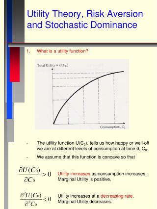
Introduction • Meyer, Jack “Choice among Distributions.” Journal of Economic Theory 14(1977): 326-36. • The general idea of the manuscript is to restrict the risk aversion coefficient for stochastic dominance to those risk aversion coefficients in a given interval r1(x)<r(x)<r2(x). Lecture 20
This problem will be solved by finding the utility function u(x) which satisfies: and minimizes Lecture 20
Given that this integral yields the expected value of F(x) minus the expected value of G(x), the minimum will be greater than zero if F(x) is preferred to G(x) by all agents who prefer F(x) to G(x). • If the minimum is less than zero, then the preference is not unanimous for all agents whose risk aversion coefficients are in the state range. • Another problem is that utility is invariant to a linear tranposition. Thus, we must stipulate that u'(0)=1. Lecture 20
The problem is then to use the control variable -u"(x)/u'(x) to maximize the objective function subject to the equation of motion Lecture 20
and the control constraints with the initial condition u'(0)=1. Lecture 20
Rewriting the problem, substituting z(x)=-u"(x)/u'(x) yields Lecture 20
The traditional Hamiltonian for this problem then becomes Following the basic Pontryagin results, a given path for control variable is optimum given three conditions: • Optimality Condition Lecture 20
Multiplier or Costate condition • Equation of Motion Lecture 20
However, in the current scenario the Hamiltonian has to be amended to account for the two inequality constraints. Specifically, Lecture 20
First examining the derivatives of the Lagrangian with respect to z(x), the control variable. We see that Lecture 20
Given the restriction that the Lagrange multipliers must be nonegative at optimum, we can see that Thus, the minimum value of the integral occurs at one of the boundaries. The question is then: What determines which boundary? Lecture 20
To examine this we begin with the Costate condition: Given this expression, we can work backward from the transversality condition. Specifically, the transversality condition for this control problem specifies that Lecture 20
Given this boundary condition, the value of l(x)u'(x) can be defined by the integral Lecture 20
Hence to complete the derivation, we must determine the value of the derivative under the integral Substituting for l'(x) from the Costate condition yields Lecture 20
Substituting for z(x) and canceling like terms yields Yielding the expression Lecture 20
Merging this result with the previous derivations, we have the infamous Theorem 5: An optimal control -u"(x)/u'(x) which maximizes Lecture 20
is given by Lecture 20
The empirical idea is then to determine whether one distribution is dominated by another distribution in the second degree with respect to a particular set of preferences. To do this we want to know if the integral switches from negative to positive within the range of risk aversion coefficients. Lecture 20
Theorem 5 states that the risk aversion which maximizes the integral will be found at one boundary or the other depending on the sign of the integral. Lecture 20
Application: • Assume that G(x)-F(x) is always nonnegative. Then for any u'(x) we consider. Thus, the optimal control for this particular F(x) and G(x) is to choose -u"(x)/u'(x) equal to its maximum possible Lecture 20
If G(x)-F(x) changes sign a finite number of times, then we know that for some x0, G(x)-F(x) does not change sign in the interval [x0,1]. Thus, the optimal solution in [x0,1] is given by the above, and once the solution in [x0,1] is known, the solution of [0,x0] can be calculated by Theorem 5. Lecture 20