Download
1 / 26
260 likes | 610 Vues
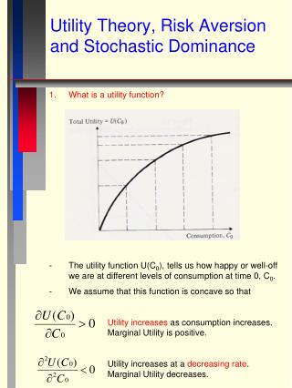
Utility Theory, Risk Aversion and Stochastic Dominance. What is a utility function? The utility function U(C 0 ), tells us how happy or well-off we are at different levels of consumption at time 0, C 0 . We assume that this function is concave so that

E N D
Utility Theory, Risk Aversion and Stochastic Dominance • What is a utility function? • The utility function U(C0), tells us how happy or well-off we are at different levels of consumption at time 0, C0. • We assume that this function is concave so that • Utility increases as consumption increases. Marginal Utility is positive. • Utility increases at a decreasing rate. Marginal Utility decreases.
2. If we consider two periods of consumption then the function U(C0, C1), is three dimensional as the figure below illustrates. - Slicing the function at some fixed level of utility “U” gives us U(C0, C1) = U. This defines an indifference curve such as the one that contains points A and B. By definition, U(C0A, C1A) = U(C0B, C1B) = U. That is, one is indifferent to receiving consumption combination (C0A, C1A) or (C0B, C1B) or any point on the curve because the utility of the each is the same and equals U.
3. If we take various slices of the function and just plot them in two dimensions (C0, C1), then we have • Here, the level of utility is increasing for indifference curves that are farther away from the origin. • The slopes of the curves at various points define the tradeoff, or marginal rate of substitution (MRS) between consumption now, C0 and consumption in the future, C1. • A particular MRS tells us the price of present consumption in terms of future consumption. Because most people prefer present to future consumption, MRS = -(1+r) where r is the interest rate. • If there is an efficient capital market, this interest rate reflects • productivity of capital goods • time preferences • production uncertainty and risk preferences
4. What is the set of consumption possibilities, (C0, C1)? This will be defined by (1) the productive potential of the capital stock and (2) the ability to borrow and lend among individuals between time periods. • if we assume that there are diminishing marginal returns to production then production possibilities will look something like the dark curve defined by X and Y below. • Borrowing and lending allow individuals to improve on pure production possibilities because at the production combination (P0, P1), they can trade amongst themselves to obtain any points along (W0, W1), the capital market line.
5. Fisher Separation: The determination of a market interest rate in the capital market separates individuals’ production decisions from their consumption decisions. • Unanimity Principal: In the graph above, production is set at (P0, P1), where the marginal rate of return on investment equals the interest rate (which is the marginal cost of funding investment). Both Investors agree that (P0, P1) is the optimal production pair even though their preferences differ considerably. Without capital markets, Investor 1 would want production at Y and Investor 2 would want production at X. • - Implication: Different shareholders of the same firm will agree on the same rule for the firm’s managers to follow: Maximize the Value (Share Price) of the Firm. • -Note that in the previous section, we saw that share price is maximized by accepting all investments up to the point where the return on the investment equals its cost of capital [r – k]=0. • 6. In equilibrium, interest rates are set in the capital market by the aggregation of individuals’ preferences. • If many people have a strong preference for C0, like Investor 1, then the weight of their preferences will push the market interest rate up and steepen the line defined by (W0, W1). This leads to a production combination with greater P0 and less P1 than before. • Question: This makes Individual 2 better off and Individual 1 worse off. Why? • The converse holds if there are more people like Individual 2.
7. Information in Interest rates and other financial prices. • -The interest rate conveys information among and between, producers and consumers. • Producers choose investment projects based on a comparison of the project’s returns to the interest rates (cost of financing). • Consumers choose consumption across time based upon the interest rate (cost of present versus future consumption). • 8. These results from Utility Theory help to explain: • Low Japanese interest rates – big savers, prefer local investments, not enough high return local investments – carry trade. • -High US interest rates – low savings, many high return investments. • Progressive tax systems • Higher tax rates for couples • Difference in anti-trust enforcement – US considers mostly consumer welfare, Europe considers “social” welfare. US approach is consistent with Finance Theory which says all economic decisions are made to support consumption. • Utility function based upon evolution – recent problems explaining some behavior with utility functions may be due to misspecification – fight-or-flight behavior may be irrational for investing.
The Consumers Problem 9. The consumer maximizes his/her utility of consumption subject to a budget constraint. Use the Lagrange Method. The Lagrangian is The first order conditions are
This is three equations in three unknowns. If we had a specific utility function we could solve for the optimal C0, C1 and . As it is we can see that Note: MRS in change in utility terms (both positive), previous graph was in terms of consumption tradeoff. Problem: Find C0, C1 for the specific function U(C0, C1) = (C0)2(C1), r=.10 and W0 = 10. First order conditions are: 2(C0)(C1) = (C0)2 = /(1+.1) C0 + C1/(1+.1) = 10 => C0 = 6.67, C1 = 3.66. Question: Why is C0 so much larger than C1? Question: How come C0 plus C1 is greater than wealth (10)? Question: This is the proper solution given these inputs but what is wrong with one of the inputs?
Utility Theory Under Uncertainty • Up until this point we have assumed • - the utility function exists • - all of the inputs are known with certainty • - perfect markets – no information or transactions costs • - consumption choice over two periods • 2. In this part, • - We will examine the requirements necessary to assure that the utility function exists. • - Handle uncertainty of the inputs. • - Utility of Wealth rather than of Consumption • - Wealth will be uncertain
3. Five axioms to assure a rational utility function exists. As before we assume more is preferred to less. • Comparability (completeness) – Individuals are able to compare all uncertain alternative outcomes, with x y, x y or x~y. • Transitivity – if x y and y z then x z. • Strong Independence – If x ~ y then one is indifferent to a gamble offering x with probability and z with probability (1 - ) or a gamble offering y with probability and z with probability (1 - ). G(x, z: ) ~ G(y, z,: ). • Measurability (continuity) – If x y z or x y z then there exists a unique , such that y ~ G(x, z,: ). This means we can make a gamble up from high and low preferred outcomes to get the equivalent of an intermediate outcome. • Ranking - If x y z andx u z then if y ~ G(x, z,: 1) and u ~ G(x, z,: 2) then if 1 > 2 then y u. If we are offered two gambles with the same outcomes but the first gamble has a greater probability of winning the bigger prize, then we will prefer the first gamble.
Properties of Utility Function to Support Expected Utility • Order Preservation – if U(x) > U(y) then x y. The proof involving gambles shows that probabilities of the gambles can be used like units of utility measure to rank the gambles. Thus there is a direct map between utility and preference. • Expected Utility can rank risky alternatives – • U[G(x, y: )] = U(x) + (1 - )U(y) • This means that we can calculate the utility of a gamble as a linear combination of the utility of the outcomes where each outcome is weighted by the probability of it occurring. This sounds trivial but is very useful. • 3. Since we assume that more is preferred to less, we know that investors will maximize their expected utility of wealth and they find this maximum using the ranking method above.
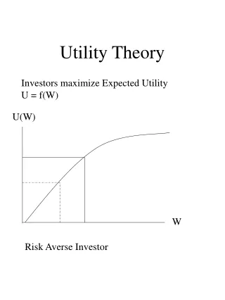
Risk Aversion • Much of the rich implications of Finance Theory relies on the assumption that most people are risk averse (utility function of wealth is concave). This is because it implies assets with different risks will have different returns. • 2. Risk Aversion defined. • U[E(W)] > E[U(W)] (generally -Jensen’s Inequality) • For a gamble with = .5 and outcomes 100 or 0, a fair bet offers an expected outcome of 50. This is also called the actuarial value of the gamble. • The risk averse gambler has a concave utility of wealth function – he prefers the sure outcome over the gamble. • U(50) > .5U(0) + .5U(100).
3. Risk Neutrality defined. U[E(W)] = E[U(W)] The risk neutral gambler has a linear utility of wealth function – he is indifferent between the sure outcome and the gamble. U(50) = .5U(0) + .5U(100).
4. Risk loving defined. U[E(W)] < E[U(W)] The risk loving gambler has a convex utility of wealth function – he prefers the gamble over the sure outcome. - Casino gamblers are assumed to be risk lovers since they expect to lose money but love the chance for a big payoff. U(50) < .5U(0) + .5U(100).
5. For a given risk-averse investor’s utility function, one can calculate the “Markowitz risk premium” or the maximum amount he would pay for insurance that gets him the expected payoff rather than have to bear the risk of the gamble. This will be the difference between expected wealth and the level of certain wealth at which he is indifferent between it and the gamble (called the certainty equivalent wealth, CEW). Problem: If U=W.5 and the gamble is G(0, 100: .5) what is the Markowitz risk premium? E[W] = 50, U[G(0, 100: .5)] = .5(0).5 + .5(100).5 = 5, At what certain wealth W is U(W) = 5 = W.5 => CEW = 25. Risk premium = E[W] – CEW = 50 – 25 = 25. Question: This assumes that the gamble represents his total wealth. Will the risk premium change if the gamble is the same but his initial wealth is 9,900 and the gamble is in addition to this amount? The cost of the gamble (CG) is the difference between current wealth W0 and the CEW. This is the maximum we would pay to take the gamble (assuming no option to receive the expected outcome as above). For the case above: CG = 0 – 25 = -25 (negative sign means we would pay 25 for the right to play the gamble) Question: What is the CG for the previous question? Can you explain the change in the size of CG?
6. The “Markowitz risk premium” is the maximum amount he would pay for insurance that gives one the expected payoff rather than have to bear the risk of the gamble. Note that this is not the amount one would pay for insurance that would leave ones level of wealth unaffected. To see this, consider the following insurance-type problem. This will be the difference between expected wealth and the level of certain wealth at which he is indifferent between it and the gamble (called the certainty equivalent wealth, CEW). Problem: If your utility function is U=W.5 and your current wealth is 1000 but there is a 50 percent chance that you will lose your job and have to use up 100 of your wealth, how much would you pay for employment insurance that would pay you the 100 if you lose your job? This is basically a gamble, G(900, 1000: .5). First, let’s look at the the Markowitz risk premium. E[W] = 950, U[G(900, 1000: .5)] = .5(900).5 + .5(1000).5 = 30.811, At what certain wealth W is U(W) = 30.811 = W.5 => CEW = 949.34. Risk premium = E[W] – CEW = 950 – 949.34 = 0.66 But the insurance premium equals expected loss plus the risk premium. Here we have E(loss) = 1000 – 950 = 50 Even a risk neutral person would pay 50. But you have a risk averse utility function so you would pay up to 50.66.
Utility-Based Measures of Risk Aversion • We will usually assume people are risk averse. This means that they have concave utility functions so that (1) their marginal utility of wealth is positive. • and (2) that the change in their marginal utility is negative. • 2. The Pratt/Arrow risk aversion measures are derived as follows. Consider an actuarially fair gamble of Z dollars (E[Z]=0). A risk premium (W, Z) must be offered to a risk averse person to make them indifferent between the gamble and its actuarial value. • E[U(W + Z)] = U[W + E(Z) - (W, Z)] • Use Taylor’s Series Approximation to approximate and expand both sides of this equation. • Note: This is similar to the Markowitz risk measure where we compare an expected wealth to a Utility of wealth.
Taylor’s approximation is a general method to evaluate a function Y = f(X) in the neighborhood around some point a. For a function of one variable we have: f(X) = f(a) + f’(a)(X-a) + f’’(a)(X-a)2/2! +….+ fn(a)(X – a)n/n! Here, because E[Z]=0, the right hand side (RHS) is U[W + E(Z) - (W, Z)] = U[W - (W, Z)]. So f(X) = U[W - (W, Z)], x = W - (W, Z), and a =W Shorten (W, Z) to just , then with Taylor’ series, U[W - ] = U(W) + U’(W)((W - )-W) + (small terms 0 because 2 assumed small) U[W - ] = U(W) - U’(W) For the LHS we have f(X) = U[W + Z], x = W + Z, and a =W. Evaluate and put the approximation inside the expectation. U[W +Z] = U(W) + U’(W)((W + Z) - W) + U’’(W)((W + Z)-W)2/2! + (small terms 0 because Z3 assumed small) E[U(W + Z)] = E[U(W) + ZU’(W) + ½Z2U’’(W)]
Because W is not random, E[U(W)] = U(W), and with E[Z] = 0, and Z2 = E[Z - E(Z)]2 = E[Z]2 because E[Z] = 0 then, E[U(W + Z)] = U(W) + ½ Z2U’’(W) Now equate the two expansion results and solve for U(W) - U’(W) = U(W) + ½ Z2U’’(W) = ½ Z2 This is the Pratt-Arrow measure of local risk premium. ARA is a measure of absolute risk aversion defined as ARA = It measures risk aversion at a given level of wealth. Relative Risk Aversion (RRA) (concerns returns) is measured by RRA = W = W[ARA]
If RRA is constant, an individual has the same risk aversion to a potential loss of a given proportion of his wealth at any wealth level (even though the dollar amount of the gamble increases with wealth). Therefore, RRA applies to rates of returns – which are proportions. Risk Tolerance = 1/ARA = Often, we judge how realistic a particular utility function is, based upon how these measures change with wealth. Many believe that most people exhibit That is, risk aversion decreases as wealth increases. Evidence from Friend and Blume (1975) shows that the power function U(W) = -Wa with a=-1 fits these restrictions well because RRA is constant and as wealth increases ARA decreases.
The Relation Between Risk Aversion and Subjective Required Probability of a Bet Using a similar approach as above to look for a risk aversion measure, one can characterize the probability of a gamble required by someone with a particular risk preference. Assume that you have wealth W and are offered a bet in which you win (or lose) $Z with probability p (1-p). Then what must p be at a minimum? You must have at least the same utility you would have without the gamble so: U(W) = pU(W+Z) + (1-p)U(W-Z) (1) Use Taylor series to approximate the two utilities on the RHS. U(W+Z) = U(W) + ZU’(W) + .5Z2(U”(W) + small U(W-Z) = U(W) - ZU’(W) + .5Z2(U”(W) + small Subst. into equation (1), ignore small terms and solve for p p = .5 + Z/4 So if you are risk neutral you only require a 50% chance but as your risk aversion or bet size Z increases you increase your required subjective probability of winning.
Small Versus Large Gambles 1. The Pratt-Arrow risk measures have assumed - small gambles - actuarially fair gambles 2. The Markowitz measure [E(W) - CEW] does not make these assumptions. 3. When gambles are small, and symmetric (actuarially fair) then both measures will give similar results, that is [E(W) - CEW] . 4. The differences result from the fact that when deriving, , we dropped terms from the Taylor series we called small. These terms are larger and more important when we have a large and asymmetric (say, skewed like the lottery) gamble. 5. Recently, researchers have found it very difficult to find a reasonable utility function that explains the way people actually behave when they confront small gambles, and when they confront large gambles - behavioral psychology.
Stochastic Dominance 1. First-Order Stochastic Dominance - asset x dominates asset y if for any outcome W, x has at least as high a probability (in some cases greater) of receiving at least W, as does y. Let Fx(W) be the cumulative probability distribution (CDF) of asset x and Gy(W) be the CDF of asset y, then Fx(W) Gy(W) for all W, and Fx(Wi) < Gy(Wi) for some Wi Assumes only that utility increases with wealth. This means that the cumulative probability distribution of y always lies to the left of that of x, they never cross. This condition is very strong and is unlikely to hold. Therefore, it is less useful than the next condition, which allows the distributions to cross.
2. Second-Order Stochastic Dominance -asset x dominates asset y if the accumulated area under the cummulative probability distribution of x, Fx(W), is smaller than the accumulated area of y’s probability distribution Gy(W) below any given level of wealth. [Gy(W) - Fx(W)]dW 0 for all W, and Fx(Wi) Gy(Wi) for some Wi Assumes that utility increases with wealth, and at a decreasing rate (risk aversion).
Second-Order Stochastic Dominance With Normal Distributions 1. Second-order stochastic (SOS) is largely applied to normal distributions because it allows us to to compare assets based solely on their means and variances. SOS is equivalent to maximizing utility for risk averse investors. The normal distribution is a symmetric distribution that is fully described by its mean and variance since its higher moments are simply functions on the mean and variance. For the concave function of a risk averter, we know that the utility value over the bottom half of a normal probability function (the part below the mean) exceeds the utility value over the top half of the normal probability function (the part above the mean). This is true because expected utility is the sum of the product of each probability and its associated utility. Distribution symmetry implies that the same probabilities multiply larger utilities losses below the mean than positive gains above the mean, so the sum of the products is negative.
3. The concept of second-order stochastic dominance with normal distributions allows us to compare all assets and say, - If asset x has a larger mean and the same variance as asset y, asset x dominates y. - If asset x has the same mean and a smaller variance than asset y, asset x dominates y. 4. These properties will help us in the next section on portfolio construction because we can eliminate assets such as y. - Best Opportunities - this will leave us with the dominant assets at each level of mean return and variance. - depending upon how risk averse we are, we will select the asset with a unique mean and variance that best suits us. 5. This will not necessarily work for non-normal distributions. Graph of mean-variance indifference curves.