Chapter 12 Risk Attitude and Utility Theory
620 likes | 1.19k Vues
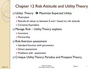
Chapter 12 Risk Attitude and Utility Theory . Utility Theory Maximize Expected Utility Motivation Rescale all values to between 0 and 1 based on risk attitude Certainty Equivalent Manage Risk – Utility Theory explains Insurance Partnership Risk Aversion assessment

Chapter 12 Risk Attitude and Utility Theory
E N D
Presentation Transcript
Chapter 12 Risk Attitude and Utility Theory • Utility Theory Maximize Expected Utility • Motivation • Rescale all values to between 0 and 1 based on risk attitude • Certainty Equivalent • Manage Risk – Utility Theory explains • Insurance • Partnership • Risk Aversion assessment • Standard function with parameters • Direct assessment • Problems with assessment • Critique Utility Theory: Paradox and Prospect Theory
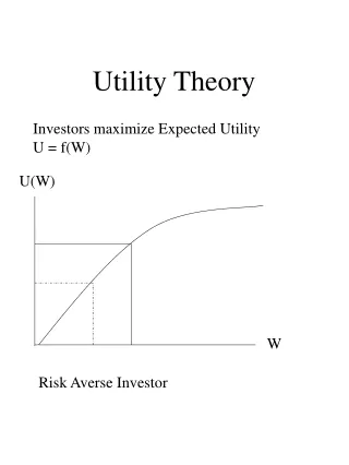
Utility Theory - Overview • Incorporates decision-maker’s risk attitude Value of alternatives cannot be captured by E(X) because risk attitude • Certainty Equivalent (CE): The payoff amount we would accept in lieu of under-going the uncertain situation, taking a gamble. • Risk Premium: A situation’s risk premium (RP) is the difference between expected payoff (EP) and certainty equivalent (CE) • Risk Aversion: CE < E(X) Concave function • Profit – prefer sure profit that is less than E(X) of a profit gamble • Cost – prefer sure cost that is higher than E(Y) of a loss gamble • Risk Prone: CE > E(X) Try for more money than average • With high guaranteed minimum, may be will to try for home run even if offered a value somewhat higher than the expected value
TV show “Deal or No Deal” – Activate WEB GAMEGame Description and Risk Attitude • Game starts with 26 suitcases, each with a dollar value ranging from $0.01 to $1M • Contestant picks one case as his to be opened at the end, and selects 6 cases to be opened immediately. As they are opened, their stored dollar value is deleted from the list. • After opening these six cases, the player is offered a sure amount or the option to keep playing. • At each the step the number of boxes to open at this stage decreases until only one at a time is opened each time. • For example, I played the game until there were 3 unopened boxes left ($25, $50,000, and $1,000,000). One of these boxes I had selected as my box. • The offer was for $220,000. This is much less than the expected value • E(X) = (1/3)(25)+ (1/3)((50,000) + (1/3)(1,000,000) = (1/3) (1,000,025) = $350,008 • If you prefer to take less than the expected value risk averse
Simple gamble (lottery) – Two OutcomesTwo boxes are left: $10,000 and $20,000. • You have a 50–50 chance of winning $10,000 or $20,000 depending upon what is in your selected box. E(X) = $15,000 • Would you accept an offer of $12,000 or continue Yes __ or No __ • Would you accept an offer of $14,500 or continue Yes __ or No __ • What is the minimum you would accept to stop the game? ___ this is Certainty Equivalent (CE) of the gamble • If the CE is less than the expected value, you are a risk averse. • Risk Premium is the difference between your CE and the expected value • Assume you would accept $12,500 • Risk Premium = E(X) – CE = $15,000 - $12,500 = $2,500 • If the CE is more than the expected value, you are a risk prone. • Gamble is a set of uncertain outcomes with probabilities • Not necessarily just 2 outcomes • All outcomes may not have the same probability.
Expected Value is Inadequate Generally Risk Averse • Extremely Rare Catastrophic Events • Law of averages no help for individual • Motivates insurance industry • Companies may self-insure up to extreme costs • Can tolerate moderate risks that are not devastating • Deductible on insurance • Large investments relative to size of company • Cannot afford the loss • Has need for certain profit more than high upside potential sell development rights
Determine function U(X) • U(X) function may be determined • Select from standard functional forms – exponential or logarithmic and estimate parameters from questions • Brute force graphing of the results of series of Certainty Equivalent responses to gambles • Assume exponential U(X) = 1-e(-x/15000) • U(20,000) = 1-e(-20000/15000) = .7364
(0.5) 0.4866 0.7364 (0.5) (0.5) $10,000 $20,000 (0.5) Calculate Expected Utility E(U(X)) and Not E(X)Assume exponential utility function for this example E(X) = 0.5($10000) + 0.5($20000) = $12,500 • Assume U(X) = 1-e(-x/15000) • U(10,000) = 1-e(-10000/15000) = 0.4866 • U(20,000) = 1-e(-20000/15000) = 0.7364 E(U(X)) = 0.5(0.487) + 0.5(0.736) = 0.6115 invert exponential function CE(0.6115) = $14,182 $14,250 would be preferred to gamble $14,000 would not be preferred
Invert function U(X) U-1(X) • 0.6115 = 1-e(-x/15000) • e(-x/15000) = 1- 0.6115 = 0.3885 • ln of both sides (-X/15000) = ln(0.3885) = -0.9455 • X = 15000 (0.9455) = 14,182 • CE of 50-50 gamble of 10,000 and 20,000 is $14,182 • Risk Premium = $15,000 - $14,182 = $818
Risk Aversion • CONCAVE for Negative (Cost) • Prefer to PAY More than expected value to be sure Cost does not get too large. • 50-50 COST Gamble $90,000 or $10,000 => prefer sure $60,000cost • Basis for Insurance Industry • CONCAVE for Maximization (Profit) • Prefer to EARN less than expected value to be sure of earning at least that profit. • 50-50 PROFIT Gamble $90,000 or $10,000 ===> would prefer sure $40,000profit to the gamble. • Basis for Selling off bank Debts such as mortgages
Risk Aversion – Concave Curve Profit Cost 0.5 for $10,000 or 0.5 for $90,000 E(X) = $50,000 Accept $40,000 = CE U(40000)=.5 Risk Premium $10,000 0.5 for -$10,000 or 0.5 for -$90,000 E(X) = -$50,000 Accept -$60,000 = CE U(60000)=.5 Risk Premium $10,000
Activity – Risk Aversion • Pay to avoid loss ___________________________________________ ___________________________________________ • Accept less profit but be sure (or more certain) of profit ___________________________________________ ___________________________________________ • Other Examples ___________________________________________ ___________________________________________ ___________________________________________ ___________________________________________
Utility Function Assessment Brute Force • Series of 3 lotteries • Obtain Certainty Equivalent of utility values of .25, .5, & .75 • Extrapolate over the range of 0 to 1. • Create your own utility function for $0M to $10M • set U(min) = 0 & U(max) = 1 • set U(0) = 0 & U(10) = 1
40.0% 0 30% Take 9.9 1.9 FALSE Take Rate Low -8 5.86 60.0% 0 50% Take 16.5 8.5 How Much Automation Investment 6.32 40.0% 0.4 30% Take 13.8 0.8 TRUE Take Rate High -13 6.32 60.0% 0.6 50% Take 23 10 Decision tree Boss Controls automation investmentNeed utility function for four values (0.8, 1.9, 8.5, 10)
(0.5) XL ≈ CE25 (0.5) CE50 (0.5) XH ≈ CE75 (0.5) CE50 (0.5) XL ≈ CE50 (0.5) XH Certainty equivalents
(0.5) (0.5) (0.5) 0 10 0 ≈ CE25 = 1.6 ≈ CE75 = 6.2 ≈ CE50 = 3.6 (0.5) (0.5) (0.5) 3.6 3.6 10 BC automation investment certainty equivalent for 0.50, 0.25, and 0.75 utility
Utility assessment for BC automation investment example Table 12‑4: Utility scores for BC automation investment
40% 0 0.13 0.13 FALSE Take Rate High 0.652 60% 0 1.0 1.0 Decision 0.657 40% 0.4 0.29 0.29 TRUE Take Rate Low 0.657 60% 0.6 0.90 0.9 Decision tree for BC automation investment using utility function 30% Take Rate 50% Take Rate Automation Investment 30% Take Rate 50% Take Rate CE: $5.142 (0.652) vs. $5.196 million (0.657)
Utility Function: Simplify Interview • Goal: simplify interview process One question for each parameter • Exponential U(x) = 1 – exp(-x/R) Constant Risk Aversion • Implies that the magnitude of cash on hand does not affect attitude towards Risk • R = Risk Tolerance • R = Sum of Money about which you are indifferent between a 50-50 chance of gaining the whole sum, R and losing the half sum, R/2
Constant Risk AversionRisk Premium is Constant R=35 U(X) = 1 – exp(-x/35)
Determine R = Risk Tolerance 50- 50 gamble to determine R Personal
Determine R = Risk Tolerance 50- 50 gamble to determine R Corporate
ENCO Project Selection An energy company will select one of two projects. If the company chooses Project A, it will undertake the development of a new power plant in one developing country. The company estimates that the investment cost will be $50 million and total revenue for five-year after the operation cost will be $80, $90, or $110 million. There is a 20% chance that the local government will take over the plant once it is finished due to some legal issues and just repay the original investment cost ($50 million). Project B also requires a $50 million investment. Total revenue for five-year after the operation cost will be $66, $80, or $90 million. In this second country, there is no chance that the government will take over this project when it is completed.
0.2 20.0% Yes 0 50 TRUE Government Take Project? Project A 34.4 -50 0.24 30.0% Low 30 80 Revenue 80.0% No 43 0 0.32 40.0% Medium 40 90 0.24 30.0% High 60 110 Project Decision Project 34.4 0 30.0% Low 16 66 FALSE Revenue Project B 28.8 -50 0 40.0% Medium 30 80 0 30.0% High 40 90 Maximize expected valueDecision tree for ENCO project selection
Figure 12.11: Cumulative risk profile for ENCO project selection Redraw diagram without student version
A utility score was calculated for each value. R= $30 million EU(Project A) = 0*20% + (0.632*30%+0.736*40%+0.865*30%)*80% = 0.595 EU(Project B) = 0.413*30%+0.632*40%+0.736*30% = 0.598
20.0% 20.0% 0 0 Yes Yes 0.000 0.000 50 50 FALSE FALSE Government Take Project? Project A Project A - - 50 50 30.0% 30.0% 0 0 0.595 Low Low 80 80 0.632 0.632 80.0% 80.0% Revenue Revenue No No 0 0 0.744 0.744 40.0% 40.0% 0 0 Medium Medium 0.736 0.736 90 90 30.0% 30.0% 0 0 High High 110 110 Project Decision Project Decision Project Project 30.0% 30.0% 0.3 0.3 Low Low 0.413 0.413 66 66 TRUE TRUE Revenue Revenue Project B Project B 0.598 0.598 - - 50 50 40.0% 40.0% 0.4 0.4 Medium Medium 80 80 0.632 0.632 30.0% 30.0% 0.3 0.3 High High 90 90 0.736 0.736 Decision tree for ENCO: using expected utility 0.865 0.598
Risk Sharing Strategies • Buy insurance • Partnerships • Example: Transmission plant by GM and Ford • Joint ventures with foreign companies • Diversification • Diversification with independent investments • Example: Dual sourcing, investment in different stocks • Diversification with dependent investments (Hedging)
Risk Sharing through Buy Insurance: Project Selection • Buy insurance against a government takeover of project A. • $4 million premium the company will receive a $10 million payment if the government takes the project. • Add new decision branch to tree as part of Project A. (top of next tree)
20.0% 0 6 60 FALSE Government Take Project? 32.400 -4 30.0% 0 26 80 80.0% Revenue 39.000 0 40.0% 0 90 36 0 30.0% 56 TRUE 110 Insurance Decicion 34.400 -50 20.0% 0.2 0 50 TRUE Government Take Project? 34.400 0 30.0% 0.24 30 80 Revenue 80.0% 43.000 0 40.0% 0.32 40 90 0.24 30.0% 60 110 Project Decision 34.400 30.0% 0 16 66 FALSE Revenue 28.800 -50 40.0% 0 80 30 30.0% 0 40 90 ENCO: insurance reporting expected value Yes • Buy Insurance Low No Medium High • Project A Yes • Do Not Buy Low No Medium High • Project Insurance Low • Project B Medium High
20.0% 0.2 TRUE 60 6 Government Take Project? -4 27.630 30.0% 0.24 80 26 80.0% Revenue 0 36.830 40% 0.32 90 36 Insurance Decision 27.630 30.0% 0.24 TRUE 110 56 -50 20.0% 0 FALSE 50 0 Government Take Project? 27.107 0 30.0% 0 30 80 80.0% Revenue 0 40.830 40.0% 0 Project Decision 90 40 27.630 30.0% 0 60 110 30.0% 0 16 66 FALSE Revenue 27.322 -50 40.0% 0 30 80 30.0% 0 40 90 ENCO : insurance option reporting CE Yes • Buy Insurance Low No Medium High • Project A Yes • Do Not Buy Low No Medium High • Project Insurance Low • Project B Medium High
Share Risk through Partnership • Concept: Commit to only a percentage of the cost (liability) and accrue the equivalent percentage of revenue • Common amongst insurance companies to reinsure and share risk of catastrophic event – Lloyd’s of London • Decision Tree Method – reduce costs and revenues proportionate to share and calculate new utility scores.
Share Risk through Partnership:Project Selection • Outside investor shares 50% of cost and benefit of each project. • By sharing the investment, the company can now be involved in more projects. Let’s evaluate a 50% share. As a result the company can invest in BOTH A and B.
Government takes away project A? TRUE Project A + 34.400 -50 Project Decision 34.400 FALSE Revenue Project B + 28.800 -50 0 30.0% 8 33 20.0% Revenue from B 14.400 25 0 40.0% 15 40 0 30.0% 20 45 FALSE Government takes away project A? 31.600 -50 0 30.0% 23 33 Revenue from B 30.0% 29.400 40 0 40.0% 30 40 0 30.0% 35 45 Revenue from A 80.0% 35.900 0 Revenue from B 40.0% + 34.400 45 Revenue from B 30.0% + 44.400 55 ENCO with 50% partnership reporting expected profit Project - Diversification Low Yes Medium High 50% of Both Projects Low Low Medium High No Medium High
FALSE Government Take Project? Project A + 27.107 -50 Project Decision Project - Diversification 29.450 FALSE Revenue Project B + 27.322 -50 0.06 30.0% Low 8 33 Revenue from B 20.0% Yes 14.032 25 0.08 40.0% Medium 15 40 0.06 30.0% High 20 45 TRUE Government Take Project A? 50% of Both Projects 29.450 -50 0.072 30.0% Low 23 33 Revenue from B 30.0% Low 29.032 40 0.096 40.0% Medium 30 40 0.072 30.0% High 35 45 Revenue from A 80.0% No 34.966 0 Revenue from B 40.0% Medium + 34.032 45 Revenue from B 30.0% High + 44.032 55 ENCO decision tree with partnership option reporting certainty equivalent
Optimize PERCENT Share of Project • Can optimize based on risk attitude • Percent share of option A • Percent share of option B • Different companies with different risk attitudes will have different optimum preferences
Phillips Petroleum and Onshore US Oil ExplorationProspect Ranking: R equal to $25 million
Following two slides not in the textbook • Impacts of the target setting on the risk attitude • Consistent with prospect theory
$47 .5 $46 OR $40 .5 Risk Attitude and TargetsComponent Cost Target $46 – Goal: Minimize Cost You are near completion on a design and are almost certain that you will be able to reach the variable cost target of $46. A suggestion comes along that by changing materials the component should be easier to manufacture with the cost dropping to $40 per part. However, time is short and there is a concern that without proper testing of Design for Manufacture the change could, in fact, increase the cost to $47 per component and miss the target. Would you make the change assuming the two outcomes were equally likely?
$47 .5 $42 OR $40 .5 Risk Attitude and TargetsComponent Cost Target $40 You are near completion on a design and are almost certain that you will NOT be able to reach the variable cost target of $40 and that the part will cost $42. A suggestion comes along that by changing materials the part should be easier to manufacture with the cost dropping to $40 per part. However, time is short and there is a concern that without proper testing of Design for Manufacture the change could, in fact, increase the cost to $47 per part and miss the target. Would you make the change assuming the two outcomes were equally likely?
Problems With Carrying Out Risk Aversion Assessment in Real-World • Managers are uncomfortable with this abstract concept • Managers are inconsistent -- Prefer ranges for CE and not specific values • People are inconsistent • risk prone for small values ( i.e. will buy lottery tickets) risk averse for large values (i.e. buy insurance) • May be risk prone if values are negative but risk averse if all values are positive and vice versa • Attitudes towards risk are influenced by artificial targets • Target secure – take no gamble to improve • Target at risk – take extreme gambles to reach target
Risk Assessment In Practice (Done Less than 10% of the time) • Howard Rule of Thumb for R in major decisions: • R = 6.4% of sales or 1.25 Net Income – Your company value? • Example: R = $1 Billion dollar investment or purchase decision for a company with over $15 Billion in sales. • First carry out analysis without Risk Aversion • Display Comparative Risk Profiles and discuss • Insert exponential function & determine whether or not the optimal solution is Sensitive to Risk Tolerance Value within a realistic range for your company. • If optimal decision can change within a reasonable range of R then assess actual utility function.
Assumptions of Utility Theory • Expectation: U(x1,p1;…;xn,pn) = p1u(x1)+…+pnu(xn) • Asset Integration: The domain of the utility function is final states (which include one’s asset position) rather than gains or losses. • Risk Aversion: u is concave (u’’< 0)
Critique of Utility Theory • Expectation Assumption - Allais paradox Problem 1: Choose between A: $1 Million with certainty B: $1 Million with probability 0.89 $5 Million with probability 0.10 0 with probability 0.01 Problem 2: Choose between X: $1 Million with probability 0.11 Y: $5 Million with probability 0.10 0 with probability 0.89 0 with probability 0.90
Critique of Utility Theory- Actual preferences • Expectation Assumption - Allais paradox Problem 1: 82% choose A A: $1 Million with certainty B: $1 Million with probability 0.89 $5 Million with probability 0.10 0 with probability 0.01 Problem 2: 83% Choose Y X: $1 Million with probability 0.11 Y: $5 Million with probability 0.10 0 with probability 0.89 0 with probability 0.90 • Conclusion: People overweight “certain” outcomes more than merely probable outcomes.
Utility Function Stability and Accuracy • Affected by mood • Quality of life QOL • Assessment of QOL living with serious disease.
Prospect Theory (Kahneman and Tversky)Example not in textbook • Value Function • Concave for gains and Convex for losses; • Steeper for losses than gains (Loss Aversion)
Prospect Theory (Kahneman and Tversky) Example not in textbook • Weighting Function (The impact of events on desirability of prospects, not merely the likelihood of events) • Overweight certainty and small probabilities; • Underweight moderate and high probabilities;
Prospect Theory (Kahneman and Tversky) Example not in textbook • Fourfold risk attitude: