Download

1 / 29
300 likes | 440 Vues
LandCaRe 2020 Dynamical and Statistical Downscaling. Ralf Lindau. Validation of CLM Precipitation by Observations Consortial Runs (Downscaling Input 18 km) are tested for 1997 – 2000 Comparison of Surface Temperatures from CLM and TERRA-Standalone

E N D
LandCaRe 2020Dynamical and Statistical Downscaling Ralf Lindau Diplomanden-Doktoranden-Seminar Bonn – 23 June 2008
Validation of CLM Precipitation by Observations Consortial Runs (Downscaling Input 18 km) are tested for 1997 – 2000 • Comparison of Surface Temperatures from CLM and TERRA-Standalone Downscaling Input is compared to downscaling output 3 Two Statistical Downscaling Methods 3.1 Spline plus Red Noise 3.2 Kriging Diplomanden-Doktoranden-Seminar Bonn – 23 June 2008
Part 1 Validation of CLM with Observations For a 4-years period (1997 – 2000) observations from Precipitation stations of DWD are compared with CLM results On average 3000 observations of daily precipitation are available in each 18 km x 18 km grid box. Diplomanden-Doktoranden-Seminar Bonn – 23 June 2008
Observations show precipitation of more than 1000 mm/a at the foothills of the Alps, in Black Forest and Bergian Land. Large areas of East Germany receive on the other hand less than 600 mm/a. The overall mean of all stations is 811 mm/a Diplomanden-Doktoranden-Seminar Bonn – 23 June 2008
In the model Middle Europe receives 1009 mm/a (left). Taking into account only such model data where observations are available, the model precipation is increased to 1156 mm/a (right). Diplomanden-Doktoranden-Seminar Bonn – 23 June 2008
On average the model overestimates the rain by 345 mm/a (44%) (left). In northern Germany the overestimation is small; in many mountain regions of southern Germany the overestimation is higher than 100%. (right) Diplomanden-Doktoranden-Seminar Bonn – 23 June 2008
Beside the absolute rain amount, the following • statistical properties of the model are validated: • PDF of rain intensity • Spatial autocorrelations Diplomanden-Doktoranden-Seminar Bonn – 23 June 2008
In the model it rains too often. Each rain class frequency is overestimated by a factor of 100.2, i.e. about 50%. No rain is observed at 49% of the days, in the model only 21% of the days are rain-free. And by the way... the overrepresentation of whole number reports is noticeable, whereas 7 and 9 tenth are seldom. In the model such priority numbers are of course unknown. + Modell 0-9 Obse Diplomanden-Doktoranden-Seminar Bonn – 23 June 2008
Frequencies of extremes are well reproduced by model. As shown on the previous slide the model produces too much light and moderate rain. However, the frequency of extreme rain amounts (20 to 100 mm/day) is in good agreement with the observations. ____ Modell 0-9 Obse Diplomanden-Doktoranden-Seminar Bonn – 23 June 2008
Spatial autocorrelation of rain The autocorrelation of the model (M) is for all distances larger than those of the observations (O). For zero-distance the obervations show a correlatin of 0.9. The decrease compared to 1 is caused by the lack of representativity of point measurements for the 18-km grid box. All other O-correlation are also reduced by this factor. TheoObs (o) are giving the corrected values. M Modell O Obse o TheoObse Diplomanden-Doktoranden-Seminar Bonn – 23 June 2008
Summary of part 1: The frequency of extreme rain events is well modelled. Also the autocorrelation is in good agreement with observations, if spurious effects of the different resolutions of model (18km) and observations (point measurements) are taken into account. It simply rains too much in the model. The rain is overestimated by about 50%. Diplomanden-Doktoranden-Seminar Bonn – 23 June 2008
Part 2 Downscaling of CLM runs (18 km) by a stand-alone version of the soil model Terra(2.8 km). Comparison of the forcing model (CLM) with high resolved output (Terra) exemplary examined by the modelled surface temperature in the Uckermark during July 2020. Diplomanden-Doktoranden-Seminar Bonn – 23 June 2008
Modelled Surface Temperature at 31 July 2020, 0:00. CLM shows warm Baltic Sea, Bornholm is detectable as cold nocturnal anomaly. The mean temperature of Uckermark is 286.5 K. At this time the high-resolution Terra output is colder (285 K). Terra CLM Diplomanden-Doktoranden-Seminar Bonn – 23 June 2008
CLM Time series of the surface temperature, exemplary for the grid point Prenzlau Midnights are marked by crosses. Considerable difference between obviously cloudy days without daily cycle and radiation days with a normal daily cycle of 15 – 20 K. Diplomanden-Doktoranden-Seminar Bonn – 23 June 2008
TERRA Time series of surface temperature at Prenzlau Smaller variations of daily cycles (10 K). The mean is at this location slightly smaller. No hot extremes above 30°C. Diplomanden-Doktoranden-Seminar Bonn – 23 June 2008
Means and total variances in space and time The temporal and spatial mean of the surface temperature over the entire July 2020 and the entire Uckermark is: CLM: 289.14 K Terra: 289.90 K Die total variance in Terra is larger compared to CLM, CLM: 16.65 K2 Terra: 23.77 K2 But attention: The increased variance cannot be interpreted as addition of small-scale variance by Terra, because the temporal variance dominates strongly: Total variance within Terra 23.77 K2 spatial variance portion 0.58 K2 small-scall spatial variance (below 18 km) 0.21 K2 Diplomanden-Doktoranden-Seminar Bonn – 23 June 2008
Structure function Terra shows a decreased variance for the same scale. This is unexpected, because: Differences between temperatures of e.g. 18 km distance should be larger in Terra compared to CLM, because the difference can be interpreted as difference of the coarse means plus the double variability within a grid box. C CLM T Terra Diplomanden-Doktoranden-Seminar Bonn – 23 June 2008
Summary Part 2 Terra modifies the original surface temperature of CLM considerably. Variation of daily cycles is smaller. Spatial variances of small scales (18 km) are reduced instead of increased. Diplomanden-Doktoranden-Seminar Bonn – 23 June 2008
Downscaling by splines Original 16 x 16 grid boxes Averaged to 4 x 4 grid boxes Is it possible to retrieve the original? Diplomanden-Doktoranden-Seminar Bonn – 23 June 2008
Splines / Idea Obviously, variance has to be added at small scales. But if variance is just added to the averaged field, nasty edges would remain visible Thus, the averaged field has to be smoothed. But simple smoothing reduces the variance. Thus, smooth the field but conserve its variance, i.e. conserve all 16 grid box averages while smoothing Diplomanden-Doktoranden-Seminar Bonn – 23 June 2008
Common Tecnique Splines fit a polynomf(x,y) to a small peace of area. The boundary conditions are continuity and differentiability In this way a smooth 2-dim surface is peacewise constructed The classic bicubic spline uses 16 coefficients With 16 boundary conditions Diplomanden-Doktoranden-Seminar Bonn – 23 June 2008
Variance conserving technique We use only 13 coefficients with 13 boundary conditions 12 + 1 Diplomanden-Doktoranden-Seminar Bonn – 23 June 2008
Variance conserving spline Original Spline retrieval Artificially coarsen Diplomanden-Doktoranden-Seminar Bonn – 23 June 2008
Adding Red Noise Spline = + Red Noise Diplomanden-Doktoranden-Seminar Bonn – 23 June 2008
Spline (last) Original Coarsen Spline Noise Result Diplomanden-Doktoranden-Seminar Bonn – 23 June 2008
Kriging Kriging is a prediction by the weighted average of surrounding data points. Existing kriging methods suppose that any new data point must reduce the predicting error. We state that an optimum selection of data points extists, which is reached if all possible new data points have negative weights. Diplomanden-Doktoranden-Seminar Bonn – 23 June 2008
Negative Kriging weights Kriging is solving this matrix: Kriging error is: Diplomanden-Doktoranden-Seminar Bonn – 23 June 2008
Precipitation from 01.01.1996 to 07.01.1996 Variance characteristics DWD Original Kriged DWD Original Kriged Constant variance reduction by the ObsError ObsError: 0.037 mm2/d2 Diplomanden-Doktoranden-Seminar Bonn – 23 June 2008
Summary 1. Attention, the rain of the Cortortial Runs might be overestimated by 50%. 2. Dynamical downscaling by TERRA results in less instead of more spatial variance. 3.1 Variance-conserving splines plus red noise are a promising tool for statistical downscaling. 3.2 The proposed kriging method subtracts exactly the observation error variance and conserves the shape of autocorrelation function. Diplomanden-Doktoranden-Seminar Bonn – 23 June 2008