Statistical Downscaling and Modelling Using Sparse Variable Selection Methods

1. Statistical Downscaling and Modelling Using Sparse Variable Selection Methods Climate Adaptation Flagship Aloke Phatak, Harri Kiiveri, Carmen Chan, Bryson Bates, & Steve Charles

2. Outline • Why Variable Selection? • Rapid Variable Elimination (RaVE) • Examples • I. Rainfall Occurrence • Sparse logistic regression • RaVE as a ‘pre-filter’ • II. Variable Selection for Extremes • Future Work 11th IMSC, 12–16 July 2010

3. Why Variable Selection? • In constructing empirical models of climatic variables, e.g., rainfall, temperature, we may have some idea of the drivers of the response of interest, but we often don’t. • Variable selection in statistical downscaling and modelling methods • ‘Expert knowledge’, model-selection criteria, and trial-and-error • NHMM – Hughes et al. (1999); Kirshner (2005) • GLM – Chandler and Wheater (2002) • Regression models (SDSM) – Wilby and Dawson, 2007; Hessami et al., 2008 • BHM for extremes – Palmer et al. (2010) • Can generally only consider a ‘small’ number of potential variables • It would be useful to have automatic variable selection methods for selecting a parsimonious set of explanatory variables from a potentially large set of e.g., gridded variables • Little work done on automatic variable selection for extreme values As always, keep in mind limitations of models from observational data 11th IMSC, 12–16 July 2010

4. Rapid Variable Elimination (RaVE) • Platforms for generating high-dimensional data have led to the situation where the number of observations, n, is much less than the number of variables, p. So, selecting a small set of explanatory variables that explains the response of interest is very challenging • Conventional methods such as best-subset selection tend to be inefficient, unstable, and slow (Breiman, 1996) • Tibshirani (1996): Seminal paper on implicit variable selection method known as LASSO (Least absolute shrinkage and selection operator) • For linear regression, LASSO boils down to a penalized least squares procedure: 11th IMSC, 12–16 July 2010

5. Rapid Variable Elimination (RaVE) • Platforms for generating high-dimensional data have led to the situation where the number of observations, n, is much less than the number of variables, p. So, selecting a small set of explanatory variables that explains the response of interest is very challenging • Conventional methods such as best-subset selection tend to be inefficient, unstable, and slow (Breiman, 1996) • Tibshirani (1996): Seminal paper on implicit variable selection method known as LASSO (Least absolute shrinkage and selection operator) • For linear regression, LASSO boils down to a penalized least squares procedure: • NB: the ridge estimator arises from: 11th IMSC, 12–16 July 2010

6. Rapid Variable Elimination (RaVE) • LASSO has a Bayesian interpretation, and that led to the use of Bayesian hierarchical priors for the vector of coefficients • In RaVE, the prior captures the assumption that although there may be many more variables than observations, the ‘true’ number of effective parameters (non-zero coefficients) is actually very small • The prior is a Normal-Gamma prior, formulated as: (Kiiveri, H.K. (2008). BMC Bioinformatics, 9:195.) 11th IMSC, 12–16 July 2010

7. Rapid Variable Elimination (RaVE) • RaVE includes LASSO as a special case ( ), and for , yields sparser models • Estimation: • The posterior of , the vector of parameters of primary interest, , the vector of parameters of secondary interest, and , given data is • By treating as missing data, we use an EM algorithm to maximize the log posterior to obtain maximum a posteriori (MAP) estimates of the vectors and given values of hyperparameters • Can be used for a wide variety of models • NB For some recent work putting regularization into a fully Bayesian framework and comparing with penalized likelihood, see • Kyung et al. (2010). Bayesian Analysis, 5 (2), 369–412 • Fahrmeir et al. (2010). Stat. Comput., 20 (2), 203–219 • Griffin and Brown (2010). Bayesian Analysis,5 (1), 171–188 11th IMSC, 12–16 July 2010

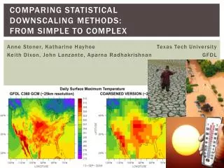
8. Example I – Rainfall Occurrence • Half-year (MJJASO) rainfall records from stations in South Australia from 1958–2006 • Atmospheric data: • NCEP-NCAR reanalysis data at 2.5° x 2.5° resolution across 7 x 8 grid • 7 potential predictor variables in each grid box: SLP, HGT and DTD at 500, 700 and 850 hPa • Total of 392 (7 x 8 x 7) potential predictors • Strategy: • Site-by-site logistic regression: • Model-building data: 1986 – 2006; Test data: 1958–1985 • Use n-fold cross-validation over a grid of k and b values • Assessment: reliability plots, ROC curves; interannual performance and wet- and dry-spell length frequencies based on simulations 11th IMSC, 12–16 July 2010

9. Example I – Study Area 11th IMSC, 12–16 July 2010

10. Example I – Selecting Hyperparameters 11th IMSC, 12–16 July 2010

11. Example I – Selected Variables (Station 2) 11th IMSC, 12–16 July 2010

12. Example I – Performance on Test Set (Station 2) 11th IMSC, 12–16 July 2010

13. Example I – Comparison With NHMM (Station 2) 11th IMSC, 12–16 July 2010

14. Example I – Comparison With NHMM (Station 2) 11th IMSC, 12–16 July 2010

15. Example 1 – Summary of Results • For all stations, RaVE selected variables in expected regions that have sensible interpretations • 11 – 18 variables selected, slight differences between stations • Results comparable to NHMM, sometimes better • Single-site, not multi-site! • Extensions: • Multi-site • Interpretation easier if spatially contiguous regions of variables were to be selected • Have also used RaVE as a ‘pre-filter’ for selecting variables for an NHMM – results comparable, slightly better • Holy grail – apply sparsity prior to NHMM? IEMSS 2010, 5 July 2010

16. Variable Selection for Extreme Values If we have a series of block maxima, and they do not change over time, then we can estimate the parameters of the GEV distribution using, say, maximum likelihood, to obtain estimates If, however, some of these parameters change over time, we have to postulate and then fit a model for this change So, in modelling the location parameter of a GEV distribution, we write: Can use RaVE to select variables in the linear predictor – need first and second derivatives of log-likelihood with respect to the linear predictor 11th IMSC, 12–16 July 2010

17. Example II • Extreme rainfall in NWWA: is it changing over time, and can we find a stable relationship with a small set of predictors? • Exploratory, use predictor(s) in more sophisticated models, ... • Wet season (NDJFMA) rainfall records from 19 stations in Kimberley and Pilbara from 1958–2007. • Atmospheric data: • NCEP-NCAR reanalysis data at 2.5° x 2.5° resolution across 11 x 9 grid • 20 potential predictor variables in each grid box: T, DTD, GPH, SH, N-S and E-W components of wind speed at 3 pressure levels; and MSLP and TT, measured on the day corresponding to the maximum rainfall • n = 47, p = 1980 • Strategy: • Diagnostic plots to determine whether extremes are changing • Variable selection using RaVE for location parameter model with constant scale and shape parameters 11th IMSC, 12–16 July 2010

18. Example II – Smoothing of Block Maxima 11th IMSC, 12–16 July 2010 Station 1 (Kimberley): NDJFMA maxima with smoothed location parameter (method of Davison and Ramesh, 2000)

19. Example II • RaVE depends on two hyper-parameters, k and b • where there is plenty of data, some form of cross-validation can be used • here, we carry out variable selection for a grid of k and b values, and then use diagnostics to assess over-fitting • With n = 47and p = 1980, how many variables would it be sensible to fit? • Rule-of-thumb: at least five observations for every parameter fitted (Huber, 1980), so no more than 5–8. • With RaVE, selecting more than about 6 – 8 variables results in severe overfitting. • Generally insensitive to value of b, but very sensitive to k. 11th IMSC, 12–16 July 2010

20. Example – Selected Variables (Station 1) Station 1 (Kimberley): 3 variables selected – DTD at 850 hPa and SH at 700 hPa. Coefficients are significant. 11th IMSC, 12–16 July 2010

21. Example Station 1 (Kimberley): Estimated location (not mean!) with pointwise 95% CI; constant scale and shape 11th IMSC, 12–16 July 2010

22. Summary • Demonstrated proof-in-principle fast variable selection for extreme values when n << p • Sensible results obtained • Picking variables at random does not yield significant coefficients, neither does using, e.g., ENSO • Much more work to be done: • Block maxima are wasteful – r-largest order statistics, point process likelihood • Multi-site models – dependency networks based on sparse regression • Interpretability – we would expect regions of variables to influence the outcome; modify the prior to force contiguous regions to be selected • Fused LASSO (Tibshirani et al. (2005) – additional constraints • Bayesian fused LASSO – Kyung et al. (2010) • Diagnostics – selection of hyperparameters k and b, goodness-of-fit measures 11th IMSC, 12–16 July 2010

23. Mathematics, Informatics and Statistics AlokePhatak Phone: +61 8 9333 6184 Email: Aloke.Phatak@csiro.au Web: www.csiro.au/cmis Thank you Contact UsPhone: 1300 363 400 or +61 3 9545 2176Email: Enquiries@csiro.au Web: www.csiro.au