Download
1 / 35
350 likes | 515 Vues
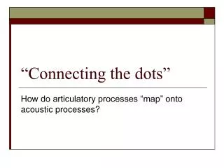
This study evaluates how articulatory processes map onto acoustic parameters in vocal production, based on the Stevens and House model (1955). We analyze key parameters such as the distance and radius of constriction within the vocal tract and their effect on formant frequencies (F1, F2, and F3). The project aims to understand how changes in vocal tract geometry influence vowel quality perception and the significance of spectral change patterns in speech. The study also examines how incorporating more variables can enhance classification accuracy and address unresolved issues in speech perception.

E N D
“Connecting the dots” How do articulatory processes “map” onto acoustic processes?
Model assumes No coupling with Nasal cavity trachea & pulmonary system Stevens and House (1955)
Model parameters Distance of major constriction from glottis (d0) Radius of major constriction (r0) Area (A) and length (l) of lip constriction A/l conductivity index Stevens and House (1955) Figure 1.
Stevens and House (1955) Figure 2.
Key Goal of Study • Evaluate the effect of systematically changing each of these three “vocal tract” parameters on F1-F3 frequency
F3 Formant Frequency (KHz) F2 F1 Figure 3. Point of Constriction (d0) (cm from glottis)
F3 F2 Formant Frequency (KHz) F1 Figure 3. Point of Constriction (d0) (cm from glottis)
NOTE Single intersection between F1 & F2 in most cases A/l Point of constriction Figure5.
A/l Figure 5. Point of constriction
A/l Point of constriction Figure 7.
∆ d0 = ∆Vfront & Vback ↑ d0 =↓ Vfront = ↑F2 ↑ d0 =↑Vback = ↓ F1 General Observations
↓ r0 =↓ F1 ↑ r0 =↑F1 When d0 ↑(anterior) ↓ r0 =↓ Vfront= ↑F2 General Observations ↑lip rounding = ↓A/l = ↓ F1 & F2
+ d0 - - r0 +
Acoustic variables related to the perception of vowel quality • F1 and F2 • Other formants (i.e. F3) • Fundamental frequency (F0) • Duration • Spectral dynamics • i.e. formant change over time
How helpful is F1 & F2? From Hillenbrand & Gayvert (1993)
How does adding more variables improve pattern classifier success? • F1, F2 + F3 • 80-85 % • F1, F2 + F0 • 80-85 % • F1, F2 + F3 + F0 • 89-90 %
Nearby vowels have different durations How about Duration?
What about Duration? Some examples
What about formant variation? Naturally spoken/hAd/ Synthesized, preserving original formant contours Synthesized with flattened formants
What about formant variation? Conclusion: Spectral change patterns do matter.
Sinewave Speech Demonstration Sinewave speech examples (from HINT sentence intelligibility test):
Selected issues that are not resolved • What do listener’s use? • Specific formants vs. spectrum envelope • What is the “planning space” used by speakers? • Articulatory • Acoustic • Auditory