DeepLab Image Segmentation: Atrous Convolutional Networks
In this article, we explore DeepLab image segmentation techniques using Atrous Convolutional Networks. Learn about semantic segmentation, DCNN layers, advantages of striding and pooling, Atrous Algorithm, and solutions for reduced resolution issues. Discover how CRFs and Fully Connected CRFs improve boundary recovery in image segmentation.

DeepLab Image Segmentation: Atrous Convolutional Networks
E N D
Presentation Transcript
Deep Segmentation Jianping Fan CS Dept UNC-Charlotte
Deep Segmentation Networks • DeepLab v1, v2, v3 • U-Nets • Fast R-CNN • Mask R-CNN
Introduction of DeepLab What is semantic image segmentation? • Partitioning an image into regions of meaningful objects. • Assignan object categorylabel.
Introduction of DeepLab DCNN and image segmentation Select maximal score class • What happens in each standard DCNN layer? • Striding • Pooling Class prediction scores for each pixel DCNN
Introduction DCNN and image segmentation • Poolingadvantages: • Invariance to small translations of the input. • Helps avoid overfitting. • Computational efficiency. • Striding advantages: • Fewer applications of the filter. • Smaller output size.
Introduction DCNN and image segmentation • What are the disadvantages for semantic segmentation? • Down-sampling causes loss of information. • The input invariance harms the pixel-perfect accuracy. • DeepLab address those issues by: • Atrousconvolution (‘Holes’ algorithm). • CRFs(Conditional Random Fields).
Up-Sampling Addressing the reduced resolution problem • Possible solution: • ‘deconvolutional’ layers (backwards convolution). • Additional memory and computational time. • Learning additional parameters. • Suggested solution: • Atrous (‘Holes’) convolution
Atrous (‘Holes’) Algorithm • Remove the down-sampling from the last pooling layers. • Up-sample the original filter by a factor of the strides:Atrous convolution for 1-D signal: • Note: standard convolution is a special case for rater=1. Introduce zeros between filter values Chen, Liang-Chieh, et al. "DeepLab: Semantic Image Segmentation with Deep Convolutional Nets, Atrous Convolution, and Fully Connected CRFs." arXiv preprint arXiv:1606.00915 (2016).
Atrous (‘Holes’) Algorithm Standard convolution Atrous convolution Chen, Liang-Chieh, et al. "DeepLab: Semantic Image Segmentation with Deep Convolutional Nets, Atrous Convolution, and Fully Connected CRFs." arXiv preprint arXiv:1606.00915 (2016).
Atrous (‘Holes’) Algorithm Filters field-of-view • Small field-of-view → accurate localization • Large field-of-view → context assimilation • ‘Holes’: Introduce zeros between filter values. • Effective filter size increases (enlarge the field-of-view of filter): • However, we take into account only the non-zero filter values: • Number of filter parameters is the same. • Number of operations per position is the same. Chen, Liang-Chieh, et al. "DeepLab: Semantic Image Segmentation with Deep Convolutional Nets, Atrous Convolution, and Fully Connected CRFs." arXiv preprint arXiv:1606.00915 (2016).
Atrous (‘Holes’) Algorithm Originalfilter Standard convolution Padded filter Atrous convolution Chen, Liang-Chieh, et al. "DeepLab: Semantic Image Segmentation with Deep Convolutional Nets, Atrous Convolution, and Fully Connected CRFs." arXiv preprint arXiv:1606.00915 (2016).
Boundary recovery • DCNN trade-off:Classification accuracy ↔ Localization accuracy • DCNN score maps successfully predict classification and rough position. • Less effective for exactoutline. Chen, Liang-Chieh, et al. "DeepLab: Semantic Image Segmentation with Deep Convolutional Nets, Atrous Convolution, and Fully Connected CRFs." arXiv preprint arXiv:1606.00915 (2016).
Boundary recovery • Possible solution: super-pixelrepresentation. • Suggested Solution: fully connected CRFs. L.-C. Chen, G. Papandreou, I. Kokkinos, K. Murphy, and A. L. Yuille, “Semantic image segmentation with deep convolutional nets and fully connected CRFs,” in ICLR, 2015. https://www.researchgate.net/figure/225069465_fig1_Fig-1-Images-segmented-using-SLIC-into-superpixels-of-size-64-256-and-1024-pixels
Conditional Random Fields Problem statement • - Random field of input observations (images) of size N. • - Set of labels. • - Random field of pixel labels. • - color vector of pixel j. • - label assigned to pixel j. • CRFs are usually used to model connections between different images. • Here we use them to model connection between image pixels! P. Krahenbuhl and V. Koltun, “Efficient inference in fully connected CRFs with Gaussian edge potentials,” in NIPS, 2011.
Probabilistic Graphical Models • Graphical Model • Factorization- a distribution over many variables represented as a product of local functions, each depends on a smaller subset of variables. C. Sutton and A. McCallum, “An introduction to Conditional Random Fields”, Foundations and Trends in Machine Learning, vol. 4, No. 4 (2011) 267–373
Probabilistic Graphical Models • Undirected vs. Directed • G(V, F, E) Directed Undirected C. Sutton and A. McCallum, “An introduction to Conditional Random Fields”, Foundations and Trends in Machine Learning, vol. 4, No. 4 (2011) 267–373
Conditional Random Fields Fully connected CRFs • Definition: • Z(X) - is an input-dependent normalization factor. • Factorization (energy function): • y - is the label assignment for pixels. P. Krahenbuhl and V. Koltun, “Efficient inference in fully connected CRFs with Gaussian edge potentials,” in NIPS, 2011. C. Sutton and A. McCallum, “An introduction to Conditional Random Fields”, Foundations and Trends in Machine Learning, vol. 4, No. 4 (2011) 267–373
Conditional Random Fields Potential functions in our case • - is the label assignment probability for pixel i computed by DCNN. • - position of pixel i. • - intensity (color) vector of pixel i. • - learned parameters (weights). • - hyper parameters (what is considered “near” / “similar”). Chen, Liang-Chieh, et al. "DeepLab: Semantic Image Segmentation with Deep Convolutional Nets, Atrous Convolution, and Fully Connected CRFs." arXiv preprint arXiv:1606.00915 (2016).
Conditional Random Fields Potential functions in our case • Bilateral kernel – nearby pixels with similar color are likely to be in the same class. • - what is considered “near” / “similar”). Pixels “nearness” Pixels color similarity Chen, Liang-Chieh, et al. "DeepLab: Semantic Image Segmentation with Deep Convolutional Nets, Atrous Convolution, and Fully Connected CRFs." arXiv preprint arXiv:1606.00915 (2016).
Conditional Random Fields Potential functions in our case • – uniform penalty for nearby pixels with different labels. • Insensitive to compatibility between labels! P. Krahenbuhl and V. Koltun, “Efficient inference in fully connected CRFs with Gaussian edge potentials,” in NIPS, 2011.
Boundary recovery Score map Belief map L.-C. Chen, G. Papandreou, I. Kokkinos, K. Murphy, and A. L. Yuille, “Semantic image segmentation with deep convolutional nets and fully connected CRFs,” in ICLR, 2015.
DeepLab • Group: • CCVL (Center for Cognition, Vision, and Learning). • Basis networks (pre-trained for ImageNet): • VGG-16(Oxford Visual Geometry Group, ILSVRC 2014 1st). • ResNet-101(Microsoft Research Asia, ILSVRC 2015 1st). • Code: https://bitbucket.org/deeplab/deeplab-public/
Simple Recipe for Classification +Localization Convolution and Pooling Fully-connected layers Softmaxloss Final conv feature map Classscores Image Fei-Fei Li & Andrej Karpathy &JustinJohnson Lecture8 - 1 Feb2016 Lecture 8 -13
Simple Recipe for Classification +Localization Fully-connected layers “Classification head” Convolution and Pooling Classscores Fully-connected layers “Regression head” Final conv feature map Boxcoordinates Image Fei-Fei Li & Andrej Karpathy &JustinJohnson Lecture8 - 1 Feb2016 Lecture 8 -14
Simple Recipe for Classification +Localization Fully-connected layers Convolution and Pooling Classscores Fully-connected layers L2 loss Final conv feature map Boxcoordinates Image Fei-Fei Li & Andrej Karpathy &JustinJohnson Lecture8 - 1 Feb2016 Lecture 8 -15
Simple Recipe for Classification +Localization Fully-connected layers Convolution and Pooling Classscores Fully-connected layers Final conv feature map Boxcoordinates Image Fei-Fei Li & Andrej Karpathy &JustinJohnson Lecture8 - 1 Feb2016 Lecture 8 -16 1 Feb2016
Per-class vs class agnosticregression Fully-connected layers Classification head: C numbers (one per class) Convolution and Pooling Classscores Class agnostic: 4 numbers (one box) Class specific: C x 4 numbers (one box per class) Fully-connected layers Final conv feature map Boxcoordinates Image Fei-Fei Li & Andrej Karpathy &JustinJohnson Lecture8 - 1 Feb2016 Lecture 8 -17 1 Feb2016
Aside: Localizing multipleobjects Want to localize exactly K objects in each image Fully-connected layers (e.g. whole cat, cat head, cat left ear, cat right ear for K=4) Convolution and Pooling Classscores Fully-connected layers K x 4numbers (one box perobject) Final conv feature map Boxcoordinates Image Fei-Fei Li & Andrej Karpathy &JustinJohnson Lecture8 - 1 Feb2016 Lecture 8 -19 1 Feb2016
Sliding Window:Overfeat Class scores: 1000 4096 4096 Winner of ILSVRC 2013 localization challenge FC FC Softmax loss Convolution +pooling FC FC FC FC Feature map: 1024 x 5 x 5 Euclidean loss Image: 3 x 221 x221 Boxes: 1000 x 4 1024 4096 Sermanet et al, “Integrated Recognition, Localization and Detection using Convolutional Networks”, ICLR 2014 Fei-Fei Li & Andrej Karpathy &JustinJohnson Lecture8 - 1 Feb2016 Lecture 8 -23 1 Feb2016
Sliding Window:Overfeat Network input: 3 x 221 x 221 Larger image: 3 x 257 x 257 Fei-Fei Li & Andrej Karpathy &JustinJohnson Lecture8 - 1 Feb2016 Lecture 8 -24
Sliding Window:Overfeat Network input: 3 x 221 x 221 Classification scores: P(cat) Larger image: 3 x 257 x 257 Fei-Fei Li & Andrej Karpathy &JustinJohnson Lecture8 - 1 Feb2016 Lecture 8 -25
Sliding Window:Overfeat Network input: 3 x 221 x 221 Classification scores: P(cat) Larger image: 3 x 257 x 257 Fei-Fei Li & Andrej Karpathy &JustinJohnson Lecture8 - 1 Feb2016 Lecture 8 -26
Sliding Window:Overfeat Network input: 3 x 221 x 221 Classification scores: P(cat) Larger image: 3 x 257 x 257 Fei-Fei Li & Andrej Karpathy &JustinJohnson Lecture8 - 1 Feb2016 Lecture 8 -27
Sliding Window:Overfeat Network input: 3 x 221 x 221 Classification scores: P(cat) Larger image: 3 x 257 x 257 Fei-Fei Li & Andrej Karpathy &JustinJohnson Lecture8 - 1 Feb2016 Lecture 8 -28
Sliding Window:Overfeat Network input: 3 x 221 x 221 Classification scores: P(cat) Larger image: 3 x 257 x 257 Fei-Fei Li & Andrej Karpathy &JustinJohnson Lecture8 - 1 Feb2016 Lecture 8 -29
Sliding Window:Overfeat Greedily merge boxes and scores (details in paper) 0.8 Network input: 3 x 221 x 221 Classification score: P (cat) Larger image: 3 x 257 x 257 Fei-Fei Li & Andrej Karpathy &JustinJohnson Lecture8 - 1 Feb2016 Lecture 8 -30
Sliding Window:Overfeat In practice use many sliding window locations and multiple scales Window positions + scoremaps FinalPredictions Box regressionoutputs Sermanet et al, “Integrated Recognition, Localization and Detection using Convolutional Networks”, ICLR 2014 Fei-Fei Li & Andrej Karpathy &JustinJohnson Lecture8 - 1 Feb2016 Lecture 8 -31
Efficient Sliding Window: Overfeat4096 4096 Class scores: 1000 FC FC Convolution +pooling FC FC FC FC Feature map: 1024 x 5 x 5 Image: 3 x 221 x221 Boxes: 1000 x 4 1024 4096 Fei-Fei Li & Andrej Karpathy &JustinJohnson Lecture8 - 1 Feb2016 Lecture 8 -32 1 Feb2016
Efficient Sliding Window:Overfeat Efficient sliding window by converting fully- connected layers into convolutions 4096 x 1 x 1 Class scores: 1000 x 1 x 1 1024 x 1 x1 Convolution +pooling 1 x 1conv 1 x 1conv 5 x 5 conv 5 x 5 conv Feature map: 1024 x 5 x 5 1 x 1conv 1 x 1conv Image: 3 x 221 x221 4096 x 1 x1 1024 x 1 x1 Box coordinates: (4 x 1000) x 1 x 1 Fei-Fei Li & Andrej Karpathy &JustinJohnson Lecture8 - 1 Feb2016 Lecture 8 -33 1 Feb2016
Efficient Sliding Window:Overfeat Training time: Small image, 1 x 1 classifier output Test time: Larger image, 2 x 2 classifier output, only extra compute at yellow regions Sermanet et al, “Integrated Recognition, Localization and Detection using Convolutional Networks”, ICLR 2014 Fei-Fei Li & Andrej Karpathy &JustinJohnson Lecture8 - 1 Feb2016 Lecture 8 -34
ImageNet Classification +Localization AlexNet: Localization method not published Overfeat: Multiscale convolutional regression with box merging VGG: Same as Overfeat, but fewer scales and locations; simpler method, gains all due to deeper features ResNet: Different localization method (RPN) and much deeper features Fei-Fei Li & Andrej Karpathy &JustinJohnson Lecture8 - 1 Feb2016 Lecture 8 -35
Computer VisionTasks Classification +Localization Instance Segmentation ObjectDetection Classification Fei-Fei Li & Andrej Karpathy &JustinJohnson Lecture8 - 1 Feb2016 Lecture 8 -36 1 Feb2016
Computer VisionTasks Classification +Localization Instance Segmentation ObjectDetection Classification Fei-Fei Li & Andrej Karpathy &JustinJohnson Lecture8 - 1 Feb2016 Lecture 8 -37 1 Feb2016
Detection asRegression? DOG, (x, y, w,h) CAT, (x, y, w,h) CAT, (x, y, w,h) DUCK (x, y, w,h) = 16numbers Fei-Fei Li & Andrej Karpathy &JustinJohnson Lecture8 - 1 Feb2016 Lecture 8 -38
Detection asRegression? DOG, (x, y, w,h) CAT, (x, y, w,h) = 8numbers Fei-Fei Li & Andrej Karpathy &JustinJohnson Lecture8 - 1 Feb2016 Lecture 8 -39
Detection asRegression? CAT, (x, y, w, h) CAT, (x, y, w, h) …. CAT (x, y, w, h) = many numbers Need variable sized outputs Fei-Fei Li & Andrej Karpathy &JustinJohnson Lecture8 - 1 Feb2016 Lecture 8 -40
Detection asClassification CAT?NO DOG?NO Fei-Fei Li & Andrej Karpathy &JustinJohnson Lecture8 - 1 Feb2016 Lecture 8 -41
Detection asClassification CAT?YES! DOG?NO Fei-Fei Li & Andrej Karpathy &JustinJohnson Lecture8 - 1 Feb2016 Lecture 8 -42
Detection asClassification CAT?NO DOG?NO Fei-Fei Li & Andrej Karpathy &JustinJohnson Lecture8 - 1 Feb2016 Lecture 8 -43