Binomial and Geometric Distributions in Statistics
230 likes | 262 Vues
Learn about binomial and geometric distributions, probability calculations, parameters, calculator functions, mean, variance, and normal approximation. Explore examples, exercises, and the importance of these distributions in statistical inference.

Binomial and Geometric Distributions in Statistics
E N D
Presentation Transcript
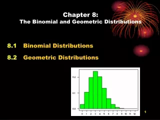
Chapter 8:The Binomial and Geometric Distributions 8.1 Binomial Distributions 8.2 Geometric Distributions
Let me begin with an example… • My best friends from Kent School had three daughters. What is the probability of having 3 girls? • We calculate this to be 1/8, assuming that the probabilities of having a boy and having a girl are equal. • But the point in beginning with this example is to introduce the binomial setting.
The Binomial Setting (p. 439) • Let’s begin by defining X as the number of girls. • This example is a binomial setting because: • Each observation (having a child) falls into just one of two categories: success or failure of having a girl. • There is a fixed number of observations (n). • The n observations are independent. • The probability of success (p) is the same for each observation.
Binomial Distributions • If data are produced in a binomial setting, then the random variable X=number of successes is called a binomial random variable, and the probability distribution of X is called a binomial distribution. • X is B(n,p) • n and p are parameters. • n is the number of observations. • p is the probability of success on any observation.
How to tell if we have a binomial setting … • Examples 8.1-8.4, pp. 440-441 • Exercise 8.1, p. 441
Binomial Probabilities—pdf • We can calculate the probability of each value of X occurring, given a particular binomial probability distribution function. • 2nd (VARS) 0:binompdf (n, p, X) • Try it with our opening example: • What is the probability of having 3 girls? • Example 8.5, p. 442 • Note conclusion on p. 443
Binomial Probabilities—cdf • Example 8.6, p. 443 • We can use a cumulative distribution function (cdf) to answer problems like this one. • Binomcdf (n, p, X)
Problems • 8.3 and 8.4, p. 445
Binomial Formulas • We can use the TI-83/84 calculator functions binompdf/cdf to calculate binomial probabilities, as we have just discussed. • We can also use binomial coefficients (p. 447). Read pp. 446-448 carefully to be able to use this alternate approach.
Homework • Read through p. 449 • Exercises: • 8.6-8.8, p. 446 • 8.12-8.13, p. 449
Mean and Standard Deviation fora Binomial Random Variable • Formulas on p. 451: • Now, let’s go back to problem 8.3, p. 445. Calculate the mean and standard deviation and compare to the histogram created.
Normal Approximation to Binomial Distributions • As the number of trials, n, increases in our binomial settings, the binomial distribution gets close to the normal distribution. • Let’s look at Example 8.12, p. 452, and Figure 8.3. • I show this because it begins to set the stage for very important concept in statistical inference—The Central Limit Theorem. • Because of the power of our calculators, however, I recommend exact calculations using binompdf and binomcdf for binomial distribution calculations.
Rules of Thumb • See box, top of page 454.
Problems • 8.15 and 8.17, p. 454 • 8.19, p. 455 • 8.27, 8.28, and 8.30, p. 461
Homework • Reading, Section 8.2: pp. 464-475 • Review: • Conditions for binomial setting • Compare to conditions for geometric setting • What’s the key difference between the two distributions? • Test on Monday
8.2 Geometric Distributions • I am playing a dice game where I will roll one die. I have to keep rolling the die until I roll a 6, then the game is over. • What is the probability that I win right away, on the first roll? • What is the probability that it takes me two rolls to get a 6? • What is the probability that it takes me three rolls to get a 6?
The Geometric Setting • This example is a geometric setting because: • Each observation (rolling a die) falls into just one of two categories: success or failure. • The probability of success (p) is the same for each observation. • The observations are independent. • The variable of interest is the number of trials required to obtain the first success.
Calculating Probability • For a geometric distribution, the probability that the first success occurs on the nth trial is: • Let’s look at Example 8.16, p. 465, and then the example calculations below that example for Example 8.15. • Why the name “geometric” for this distribution? • See middle of page 466.
“Calculator Speak” • Notice that we do not have an “n” present in the following calculator commands … that’s the point of a geometric distribution!
Exercises:8.38, p. 4688.43 (b&c), p. 474 -- See example 8.15, p. 465
Homework • Read through the end of the chapter. • Problems: • 8.36, p. 463 • 8.39, p. 468 • 8.46, p. 474 • 8.55 and 8.56, p. 479 • 8.1-8.2 Quiz Friday
Chapter 8 Review Problems • pp. 480-482: • 8.60 • 8.61 • 8.62 • 8.63