Chapter 8 Binomial and Geometric Distributions
390 likes | 676 Vues
Chapter 8 Binomial and Geometric Distributions. 8.1 Binomial Random Variables Binomial Distribution. Binomial and Geometric Random Variables. Learning Objectives. After this section, you should be able to… DETERMINE whether the conditions for a binomial setting are met

Chapter 8 Binomial and Geometric Distributions
E N D
Presentation Transcript
Chapter 8Binomial and Geometric Distributions • 8.1 Binomial Random Variables • Binomial Distribution
Binomial and Geometric Random Variables Learning Objectives After this section, you should be able to… • DETERMINE whether the conditions for a binomial setting are met • COMPUTE and INTERPRET probabilities involving binomial random variables • CALCULATE the mean and standard deviation of a binomial random variable and INTERPRET these values in context • CALCULATE probabilities involving geometric random variables
Binomial and Geometric Random Variables • Binomial Random Variables – ESP To test whether someone has ESP, choose one of four cards at random – a star, wave, cross, or Circle. Ask the person to identify the card without seeing it. Do this a total of 50 times, and see how many cards the person identifies correctly. • Chance process: choose a card at random • Outcome of interest: person identifies card correctly • Random Variable X: number of correct identifications
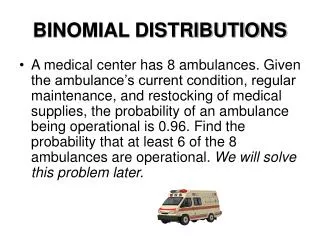
Binomial and Geometric Random Variables • Binomial Random Variables – Shipping Claims A shipping company claims that 90% of its shipments arrive on time. To test this claim, take a random sample of 100 shipments made by the company last month and see how many arrived on time. • Chance process: Randomly select a shipment and check when it arrived • Outcome of interest: arrived on time • Random Variable Y: number of on-time shipments These are binomial random variables because we are counting the number of times the outcome of interest occurs in a fixed number of repetitions.
Binomial and Geometric Random Variables • Geometric Random Variables – Pass the Pigs In the game of Pass the Pigs, a player rolls a pair of pig-shaped dice. On each roll, the player earns points according to how the pigs land. If the player gets a “pig out” in which the two pigs land on opposite sides, she loses all points earned in that round and must pass the pigs to the next player. A player can choose to stop rolling at any point during her turn and keep the points that she has earned before passing the pigs. • Chance process: roll the pig dice • Outcome of interest: pig out • Random Variable T: number of rolls until the player pigs out This is a geometric random variable because we are counting the number of repetitions of the chance process needed for the outcome of interest to occur.
Binomial and Geometric Random Variables • Binomial Settings Sometimes we are performing repeated trials of the same chance process. The number of trials is fixed in advance, and the outcome of one trial has no effect on the outcome of any other trial. We are interested in the number of times that a specific event occurs. Our chances of getting a “success” are the same on each trial. If so, we have a binomial setting. • Toss a coin 5 times. Count the number of heads. • Spin a roulette wheel 8 times. Record how many times the ball lands in a red slot. • Take a random sample of 100 babies born in U.S. hospitals today. Count the number of females. • Look at a packet of 20 tomato plant seeds. Plant them and determine how many germinate. (Assume independence.)
Binomial and Geometric Random Variables • Binomial Settings When the same chance process is repeated several times, we are often interested in whether a particular outcome does or doesn’t happen on each repetition. In some cases, the number of repeated trials is fixed in advance and we are interested in the number of times a particular event (called a “success”) occurs. If the trials in these cases are independent and each success has an equal chance of occurring, we have a binomial setting. Definition: A binomial setting arises when we perform several independent trials of the same chance process and record the number of times that a particular outcome occurs. The four conditions for a binomial setting are • Binary? The possible outcomes of each trial can be classified as “success” or “failure.” B • Independent?Trials must be independent; that is, knowing the result of one trial must not have any effect on the result of any other trial. I N • Number?The number of trials n of the chance process must be fixed in advance. S • Success?On each trial, the probability p of success must be the same.
Binomial and Geometric Random Variables • Binomial Settings Identify whether the given random variable has a binomial distribution. If so, determine its BINS. • Put the names of all of the students in your class in a hat. Mix them up, and draw four names without looking. Let Y = the number whose last names have more than six letters. • Exactly 10% of students in a school are left-handed. Select students at random from the school, one at a time, until you find one who is left-handed. Let V = the number of students chosen. •Exactly 10% of students in a school are left-handed. Select 15 students at random from the school and define W = the number who are left-handed.
Binomial and Geometric Random Variables • Binomial Settings Identify whether the given random variable has a binomial distribution. If so, determine its BINS. • Genetics says that children receive genes from each of their parents independently. Each child of a particular pair of parents has probability 0.25 of having type O blood. Suppose these parents have 5 children. Let X = the number of children with type O blood. • Shuffle a deck of cards. Turn over the first 10 cards, one at a time. Let Y = the number of aces observed. •Shuffle a deck of cards. Turn over the top card. Put the card back in the deck, and shuffle again. Repeat this process until you get an ace. Let W = the number of cards required.
Binomial and Geometric Random Variables • Binomial Settings Identify whether the given random variable has a binomial distribution. If so, determine its BINS. • Roll a fair die 10 times and let X = the number of sixes. • Shoot a basketball 20 times from various distances on the court. Let Y = number of shots made. Observe the next 100 cars that go by and let C = color.
Binomial and Geometric Random Variables • Binomial Settings Identify whether the given random variable has a binomial distribution. If so, determine its BINS. • Shuffle a deck of cards. Turn over the top card. Put the card back in the deck and shuffle again. Repeat this process 10 times. Let X = the number of hearts you observe. Choose 3 students from the class. Let Y = the number who are over 6 feet tall. Flip a coin. If it’s heads, roll a 6-sided die. If it’s tails, roll an 8-sided die. Repeat this process 5 times. Let W = the number of 5s rolled.
Binomial and Geometric Random Variables • Binomial Random Variable Consider tossing a coin n times. Each toss gives either heads or tails. Knowing the outcome of one toss does not change the probability of an outcome on any other toss. If we define heads as a success, then p is the probability of a head and is 0.5 on any toss. The number of heads in n tosses is a binomial random variable X. The probability distribution of X is called a binomial distribution. Definition: The count X of successes in a binomial setting is a binomial random variable. The probability distribution of X is a binomial distribution with parameters n and p, where n is the number of trials of the chance process and p is the probability of a success on any one trial. The possible values of X are the whole numbers from 0 to n. Note: When checking the Binomial condition, be sure to check the BINS and make sure you’re being asked to count the number of successes in a certain number of trials!
Binomial and Geometric Random Variables • Binomial Probabilities In a binomial setting, we can define a random variable (say, X) as the number ofsuccesses in n independent trials. We are interested in finding the probability distribution of X. Example Each child of a particular pair of parents has probability 0.25 of having type O blood. Genetics says that children receive genes from each of their parents independently. If these parents have 5 children, the count X of children with type O blood is a binomial random variable with n = 5 trials and probability p = 0.25 of a success on each trial. In this setting, a child with type O blood is a “success” (S) and a child with another blood type is a “failure” (F). What’s P(X = 0)? P(FFFFF) = (0.75)(0.75)(0.75)(0.75)(0.75) = (0.75)5 = 0.2373 Therefore, P(X = 0) = (0.75)5 = 0.2373
Binomial and Geometric Random Variables • Binomial Probabilities In a binomial setting, we can define a random variable (say, X) as the number ofsuccesses in n independent trials. We are interested in finding the probability distribution of X. Example Each child of a particular pair of parents has probability 0.25 of having type O blood. Genetics says that children receive genes from each of their parents independently. If these parents have 5 children, the count X of children with type O blood is a binomial random variable with n = 5 trials and probability p = 0.25 of a success on each trial. In this setting, a child with type O blood is a “success” (S) and a child with another blood type is a “failure” (F). What’s P(X = 1)? P(SFFFF) = (0.25)(0.75)(0.75)(0.75)(0.75) = (0.25)(0.75)4 = 0.0791 However, there are a number of different arrangements, each of which have a probability of 0.0791, in which 1 out of the 5 children have type O blood: SFFFF FSFFF FFSFF FFFSF FFFFS Verify that in each arrangement, P(X = 1) = (0.25)(0.75)4 = 0.0791 Therefore, P(X = 1) = 5(0.25)(0.75)4 = 0.39551
Binomial and Geometric Random Variables • Binomial Probabilities In a binomial setting, we can define a random variable (say, X) as the number ofsuccesses in n independent trials. We are interested in finding the probability distribution of X. Example Each child of a particular pair of parents has probability 0.25 of having type O blood. Genetics says that children receive genes from each of their parents independently. If these parents have 5 children, the count X of children with type O blood is a binomial random variable with n = 5 trials and probability p = 0.25 of a success on each trial. In this setting, a child with type O blood is a “success” (S) and a child with another blood type is a “failure” (F). What’s P(X = 2)? P(SSFFF) = (0.25)(0.25)(0.75)(0.75)(0.75) = (0.25)2(0.75)3 = 0.02637 However, there are a number of different arrangements in which 2 out of the 5 children have type O blood: SSFFF SFSFF SFFSF SFFFS FSSFF FSFSF FSFFS FFSSF FFSFS FFFSS Verify that in each arrangement, P(X = 2) = (0.25)2(0.75)3 = 0.02637 Therefore, P(X = 2) = 10(0.25)2(0.75)3 = 0.2637
Binomial and Geometric Random Variables • Binomial Probabilities In a binomial setting, we can define a random variable (say, X) as the number ofsuccesses in n independent trials. We are interested in finding the probability distribution of X. Example In many games involving dice, rolling doubles is desirable. Rolling doubles means that the outcomes of two dice are the same, such as 1 and 1, or 5 and 5. The probability of rolling doubles when rolling two dice is 6/36, or 1/6. If X = the number of doubles in 4 rolls of two dice, then X is binomial with n = 4 and p = 1/6. What’s P(X = 0)? P(FFFF) = (5/6)(5/6)(5/6)(5/6) = (5/6)4 = 0.48225 Therefore, P(X = 0) = (5/6)4 = 0.48225
Binomial and Geometric Random Variables • Binomial Probabilities In a binomial setting, we can define a random variable (say, X) as the number ofsuccesses in n independent trials. We are interested in finding the probability distribution of X. Example In many games involving dice, rolling doubles is desirable. Rolling doubles means that the outcomes of two dice are the same, such as 1 and 1, or 5 and 5. The probability of rolling doubles when rolling two dice is 6/36, or 1/6. If X = the number of doubles in 4 rolls of two dice, then X is binomial with n = 4 and p = 1/6. What’s P(X = 1)? P(FFFF) = (1/6)(5/6)(5/6)(5/6) = (1/6)(5/6)3 = 0.09645 However, there are a number of different arrangements in which 1 out of the 4 rolls is a double: SFFF FSFF FFSF FFFS Verify that in each arrangement, P(X = 1) = (1/6)(5/6)3 = 0.09645 Therefore, P(X = 1) = 4(1/6)(5/6)3 = 0.3858
Binomial and Geometric Random Variables • Binomial Coefficient Note, in the example about the family and Type O blood, any one arrangement of 2 S’s and 3 F’s had the same probability. This is true because no matter what arrangement, we’d multiply together 0.25 twice and 0.75 three times. We can generalize this for any setting in which we are interested in k successes in n trials. That is, Definition: The number of ways of arranging k successes among n observations is given by the binomial coefficient for k = 0, 1, 2, …, n where n! = n(n – 1)(n – 2)•…•(3)(2)(1) and 0! = 1. Some people prefer the notation nCk for the binomial coefficient. This formula will be on the AP Exam formula sheet!
Binomial and Geometric Random Variables • Binomial Probability The binomial coefficient counts the number of different ways in which k successes can be arranged among n trials. The binomial probability P(X = k) is this count multiplied by the probability of any one specific arrangement of the k successes. Binomial Probability If X has the binomial distribution with n trials and probability p of success on each trial, the possible values of X are 0, 1, 2, …, n. If k is any one of these values, Number of arrangements of k successes Probability of n-k failures Probability of k successes
Binomial and Geometric Random Variables • Binomial Coefficients on the Calculator Calculate a binomial coefficient like as follows: TI-83/84: Type 5, press MATH, arrow over to PRB, choose 3:nCr, and press ENTER Then type 2, and press ENTER again. TI-89: From the home screen, press 2nd 5 (MATH), choose 7: Probability, 3: nCr Complete the command nCr(5, 2) and press ENTER
Example: Inheriting Blood Type Each child of a particular pair of parents has probability 0.25 of having blood type O. Suppose the parents have 5 children (a) Find the probability that exactly 3 of the children have type O blood. Let X = the number of children with type O blood. We know X has a binomial distribution with n = 5and p = 0.25. (b) Should the parents be surprised if more than 3 of their children have type O blood? To answer this, we need to find P(X > 3). Since there is only a 1.5% chance that more than 3 children out of 5 would have Type O blood, the parents should be surprised!
Example: Rolling Doubles When rolling two dice, the probability of rolling doubles is 1/6. Suppose that a game player rolls the dice 4 times, hoping to roll doubles. (a) Find the probability that the player gets doubles twice in four attempts. Let X = number of doubles. X has a binomial distribution with n = 4 and p = 1/6. (b) Should the player be surprised if he gets doubles more than twice in 4 attempts? To answer this, we need to find P(X > 2). Since there is only a 1.6% chance that the player will roll doubles more than twice in 4 attempts, he should be surprised.
Binomial and Geometric Random Variables • Binomial Probability on the Calculator Binompdf(n,p,k) computes P(X = k) Binomcdf(n,p,k) computes P(X < k) TI-83/84: These commands are found in the distributions menu (2nd/VARS) TI-89: These commands are found in CATALOG under Flash Apps For the parents having n = 5 children, each with the probability p = 0.25 of type O blood: P(X = 3) = binompdf(5, 0.25, 3) = 0.08789 To find P(X > 3) = 1 – P(X < 3) = 1 – binomcdf(5, 0.25, 3) = 0.01563
CHECK YOUR UNDERSTANDING To introduce his class to binomial distributions, Mr. Leonard gives a 10-item, multiple choice quiz. The catch is, students must simply guess an answer (A through E) for each question. Mr. Leonard uses his computer’s random number generator to produce the answer key, so that each possible answer has an equal chance to be chosen. Christiana is one of the students in this class. Let X = the number of Christiana’s correct guesses. (a) Show that X is a binomial random variable. Check the BINS. This is a binomial setting. X is a binomial random variable with n = 10 and p = 0.20. (b) Find P(X = 3). Explain what this means. P(X = 3) = 0.2013. There is a 20% chance that Christiana will answer exactly 3 questions correctly. (c) To get a passing score on the quiz, a student must guess correctly at least 6 times. Would you be surprised if Christiana earned a passing score? Compute the appropriate probability to support your answer. P(X > 5) = 0.0064. Since there is only a 0.64% chance that a student will pass, we would be surprised if Christiana passed.
Binomial and Geometric Random Variables • AP EXAM ERROR ALERT! When using the complement rule for discrete probability distributions such as the binomial distribution, students often have trouble identifying the correct complementary event. For example, if students are asked to find P(X ≥ 2), many will calculated 1 – P(X ≤ 2) rather than 1 – P(X ≤ 1). To avoid this mistake, write out the possible values of X, circle the ones you want to find the probability of, and cross out the remaining values that make up the complementary event.
Binomial and Geometric Random Variables • AP EXAM ERROR ALERT! Don’t use “calculator speak” when showing your work on free-response questions. Writing binompdf(5, 0.25, 3) = 0.08789 will not earn you full credit for a binomial probability calculation. At the very least, you must indicate what each of those calculator inputs represents. For example, “I used binompdf(5, 0.25, 3) on my calculator with n = 3, p = 0.25, and k = 3.” Better yet, show the binomial probability formula (it will be on your formula sheet!) with those numbers plugged in.
Binomial and Geometric Random Variables • Mean and Standard Deviation of a Binomial Distribution We describe the probability distribution of a binomial random variable just like any other distribution – by looking at the shape, center, and spread. Consider the probability distribution of X = number of children with type O blood in a family with 5 children. Shape: The probability distribution of X is skewed to the right. It is more likely to have 0, 1, or 2 children with type O blood than a larger value. Center: The median number of children with type O blood is 1. Based on our formula for the mean: Spread: The variance of X is The standard deviation of X is
Binomial and Geometric Random Variables • Mean and Standard Deviation of a Binomial Distribution Notice, the mean µX= 1.25 can be found another way. Since each child has a 0.25 chance of inheriting type O blood, we’d expect one-fourth of the 5 children to have this blood type. That is, µX= 5(0.25) = 1.25. This method can be used to find the mean of any binomial random variable with parameters n and p. Mean and Standard Deviation of a Binomial Random Variable If a count X has the binomial distribution with number of trials n and probability of success p, the mean and standard deviation of X are Also included in the AP Exam formula sheet. Note: These formulas work ONLY for binomial distributions. They can’t be used for other distributions!
Example: Bottled Water versus Tap Water The 21 teachers at Ms. Raskin’s Nerd Camp did the Bottled Water activity. If we assume the teachers in this class cannot tell tap water from bottled water, then each has a 1/3 chance of correctly identifying the different type of water by guessing. Let X = the number of teachers who correctly identify the cup containing the different type of water. Find the mean and standard deviation of X. Since X is a binomial random variable with parameters n = 21 and p = 1/3, we can use the formulas for the mean and standard deviation of a binomial random variable. If the activity were repeated many times with groups of 21 students who were just guessing, the number of correct identifications would differ from 7 by an average of 2.16. We’d expect about one-third of his 21 students, about 7, to guess correctly.
Example: Diet Soda vs. Regular Soda The makers of a diet soda claim that its taste is indistinguishable from the full-calorie version of the same soda. To investigate, Sarah prepared small samples of each type of soda in identical cups. Then she had volunteers taste each soda in a random order and try to identify which was the diet soda and which was the regular. Overall, 23 of the 30 subjects made the correct identification. Find the mean and standard deviation of X. Since X is a binomial random variable with parameters n = 30 and p = 0.5, we can use the formulas for the mean and standard deviation of a binomial random variable. If the activity were repeated many times with groups of 30students who were just guessing, the number of correct identifications would differ from 15 by an average of 2.74. We’d expect about 15 people to guess correctly. Of the 30 volunteers, 23 made correct identifications. Does this give convincing evidence that the volunteers can taste the difference between diet and regular soda? P(X ≥ 23) = 1 – P(X ≤ 22 = 1 – binomcdf(30, 0.5, 22) = 1 – 0.9974 = 0.0026 There is a very small chance that there would be 23 or more correct guesses.
Binomial and Geometric Random Variables • Example: Diet Soda vs. Regular Soda Here is the probability distribution for the number for correct guesses in Ms. Raskin’s summer class. Where have you previously seen this graph?
CHECK YOUR UNDERSTANDING To introduce his class to binomial distributions, Mr. Leonard gives a 10-item, multiple choice quiz. The catch is, students must simply guess an answer (A through E) for each question. Mr. Leonard uses his computer’s random number generator to produce the answer key, so that each possible answer has an equal chance to be chosen. (a) Find μx. Interpret this value in context. μx = 2. We would expect the average student to get 2 answers correct. (b) Find σx. Interpret this value in context. σx = 1.265. We would expect individual students’ scores to vary from a mean of 2 by an average of 1.265 correct answers. (c) What’s the probability that the number of Christiana’s correct guesses is more than 2 standard deviations above the mean? Show your method. P(X > 4.53) = 1 – P(X ≤ 4) = 0.0328
Binomial and Geometric Random Variables • Binomial Distributions in Statistical Sampling The binomial distributions are important in statistics when we want to make inferences about the proportion p of successes in a population. Suppose 10% of CDs have defective copy-protection schemes that can harm computers. A music distributor inspects an SRS of 10 CDs from a shipment of 10,000. Let X = number of defective CDs. What is P(X = 0)? Note, this is not quite a binomial setting. Why? The actual probability is Using the binomial distribution, In practice, the binomial distribution gives a good approximation as long as we don’t sample more than 10% of the population. Sampling Without Replacement Condition When taking an SRS of size n from a population of size N, we can use a binomial distribution to model the count of successes in the sample as long as
Normal Approximation of Binomial Distribution • Normal Approximation • * Check SHOW PROBABILITY and set values from 3-5 • * Change values for N and notice the difference in actual versus approximated probability • * Change values for p and notice the difference in actual versus approximated probability • When is this approximation accurate enough to be useful??? Mathshepherd.com
Binomial and Geometric Random Variables • Normal Approximation for Binomial Distributions As n gets larger, something interesting happens to the shape of a binomial distribution. The figures below show histograms of binomial distributions for different values of n and p. What do you notice as n gets larger? Normal Approximation for Binomial Distributions Suppose that X has the binomial distribution with n trials and success probability p. When n is large, the distribution of X is approximately Normal with mean and standard deviation As a rule of thumb, we will use the Normal approximation when n is so large that np ≥ 10 and n(1 – p) ≥ 10. That is, the expected number of successes and failures are both at least 10.
Example: Attitudes Toward Shopping Sample surveys show that fewer people enjoy shopping than in the past. A survey asked a nationwide random sample of 2500 adults if they agreed or disagreed that “I like buying new clothes, but shopping is often frustrating and time-consuming.” Suppose that exactly 60% of all adult US residents would say “Agree” if asked the same question. Let X = the number in the sample who agree. Estimate the probability that 1520 or more of the sample agree. 1) Verify that X is approximately a binomial random variable. B: Success = agree, Failure = don’t agree I: Because the population of U.S. adults is greater than 25,000, it is reasonable to assume the sampling without replacement condition is met. N: n = 2500 trials of the chance process S: The probability of selecting an adult who agrees is p = 0.60 2) Check the conditions for using a Normal approximation. Since np = 2500(0.60) = 1500 and n(1 – p) = 2500(0.40) = 1000 are both at least 10, we may use the Normal approximation. 3) Calculate P(X ≥ 1520) using a Normal approximation.
Example: Teens and debit cards In a survey of 506 teenagers aged 14 to 18, subjects were asked if they had a debit card. Suppose that exactly 10% of teens aged 14 to 18 have debit cards. Let X = the number of teens in a random sample of size 506 who have a debit card. 1) Verify that the distribution of X is approximately binomial. B: Yes I: No, since we are sampling without replacement. However, since the sample size (n = 506) is much less than 10% of the population, the responses will be very close to independent. N: n = 506 S: The probability of selecting a teen with a debit card is p = 0.60 2) Check the conditions for using a Normal approximation. Since np = 506(0.10) = 50.6 and n(1 – p) = 506(0.90) = 455.5 are both at least 10, we may use the Normal approximation. 3) Calculate P(X ≤ 40) using a Normal approximation. P(X ≤ 40) = normalcdf(-9999, 40, 50.6, 6.75) = 0.058
Example: Dead Batteries Almost everyone has a drawer that holds miscellaneous batteries of all sizes. Suppose that your drawer contains 8 AAA batteries but only 6 of them are good. You need to choose 4 for your graphing calculator. If you randomly select 4 batteries, what is the probability that all 4 of the batteries you choose will work? The actual probability is 0.2143, not 0.3164.P(X = 4) = (0.75)4(0.25)4 = 0.3164. Why isn’t the answer 0.3164? Since we are sampling without replacement, the selections of batteries aren’t independent. We can ignore this problem if the sample we are selecting is less than 10% of the population. However, in this case, we are sampling 50% of the population, so it is not reasonable to ignore the lack of independence and use the binomial distribution. This explains why the binomial probability is so different from the actual probability.
President Bush’s morning security briefing is wrapping up. Defense Secretary Donald Rumsfeld is concluding his part and says, "Finally, three Brazilian soldiers were killed yesterday near Baghdad." • "OH MY GOD!" shrieks Bush, and he buries his head in his hands for a seemingly interminable 30 seconds. • Stunned at the unexpected display of emotion, the President's staff sits speechless, not sure how to react. Finally, Bush looks up and asks Rumsfeld, "How many is a brazillion?”