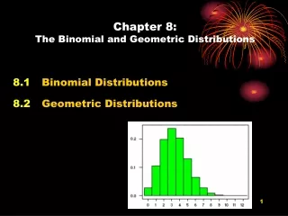
Chapter 8 The Binomial and Geometric Distributions

1. Chapter 8 The Binomial and Geometric Distributions

2. Activity 8 – page 438 • Before we simulate this event, how would we determine the probability of a couple having 3 girl children? • What is the theoretical probability of the family having all 3 children be girls?

3. Binomial Probabilities • Tossing a coin to see which football team gets the choice of kicking off or receiving the to begin the game. • P(winning the coin toss)=.5 • A basketball player shoots a free throw; the outcomes of interest are {makes free throw, misses free throw} • P(making free throw) = ? • A young couple prepares for their first child; the outcomes of interest are {boy, girl} • P(boy)=.5 • A manufacturer inspects items off of an assembly line; outcomes of interest are {defective, not defective}

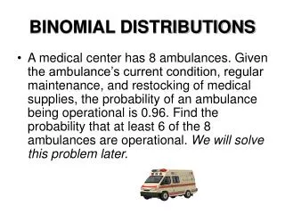
4. Binomial Setting • 1. Each observation falls into one of just two categories, which for convenience we call “success” and “failure”. • 2. There is a fixed number of trials. • 3.The n observations are all independent. That is, knowing the result of one observation tells you nothing about the other observations. • 4. The probability of success, call it p, is the same for each observation. • 5. We are looking usually for the probability of r successes out of the n trials.

5. Binomial Random Variable • The distribution of the count X of successes in the binomial setting is the binomial distribution with parameters n and p. • The parameter n is the number of observations, and p is the probability of a success on any one observation. • The possible values of X are the whole numbers 0 to n. • As an abbreviation, we say that X is B(n,p)

6. Example 8.1 • Read and discuss with a neighbor.

7. Example 8.2 • Read and discuss with a neighbor.

8. Example 8.3 • Read and discuss with a neighbor.

9. Example 8.4 • Read and discuss with a neighbor. Be prepared to explain to the class.

10. Example 8.5 • Read and discuss with a neighbor. Be prepared to discuss with the class.

11. Binompdf & Binomcdf • 2nd DISTR • binompdf (n,p,r) • Binompdf (10,.1,1)= .387420489. The exact probability for 1 trial out of 10 tries being successful when p=.1. • Binomcdf (n,p,r) cumulative probability. Probability of up to r successes out of n trials.

12. Example 8.6 • Read and discuss with a neighbor. Be prepared to discuss with the class. • How would you do this with the calculator?

13. Example 8.7 • Read and discuss with a neighbor. Be prepared to discuss with the class.

14. Example 8.8 • Read and discuss with a neighbor. Be prepared to discuss with the class.

15. Example 8.9 • Read and discuss with a neighbor. Be prepared to discuss with the class.

16. Binomial Probability • If X has the binomial distribution with n observations and probability p of success on each observation, the possible values of X are 0, 1, 2, …, n. If k is any of those values,

17. Example 8.10 • Read and discuss with a neighbor. Be prepared to discuss with the class.

18. Binomial Mean and Standard Deviation

19. The Normal approximation to Binomial Distributions • As the number of trials n gets larger and larger, the binomial distribution gets closer and closer to a normal distribution.

20. The Normal approximation to Binomial Distributions • Two criteria must be met to approximate use the normal curve as an approximation of a binomial distribution. • n(p) > 10 and n(1-p) >10

21. Example 8.12 • Read and discuss with a neighbor. Be prepared to discuss with the class.

22. Example 8.13 • Read and discuss with a neighbor. Be prepared to discuss with the class.

23. Normal Approximation for Binomial Distributions • Suppose that a count X has the binomial distribution with n trials and success probability p. When n is large, the distribution is approximately normal, N (np, )

24. Technology Toolbox • How can we get the calculator to draw a binomial distribution for us? Pg. 456 • Do problems through number 1 – 20 and 27 – 34.

25. 8.2 Geometric Distributions • Geometric Setting • 1. Each observation falls into one of just two categories, which for convenience we call “success” and “failure”. • 2. The probability of success, call it p, is the same for each observation. • 3. The observations are all independent. • 4. The variable of interest is the number of trials required to obtain the first success.

26. Example 8.15 • Read and be prepared to explain to the class.

27. Example 8.16 • Read and be prepared to explain to the class.

28. How to Calculate Geometric Probabilities • If X has a geometric distribution with probability p of success and (1 – p) of failure on each observation, the possible values of X are 1, 2, 3, … If n is any one of these values, the probability that the first success occurs on the nth trial is

29. Example 8.17 • Read and be prepared to explain to the class.

30. Expected Value and Variance of Geometric Distributions • If X is a geometric random variable with probability of success p on each trial, then the mean, or expected value, of the random variable, that is , the expected number of trials required to get the first success is • The variance of X is

31. Example 8.18 • Read and be prepared to explain to the class.

32. Example 8.19 • Read and be prepared to explain to the class.

33. Calculator Commands • geometpdf(p,r) will give you the probability of the first success happening exactly on the rth trial. • geometcdf (p,r) is the cumulative probability of the 1st success happening within r trials.