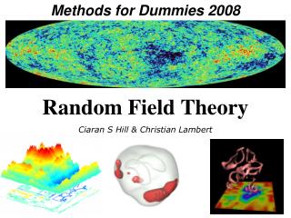
Random Field Theory
Methods for Dummies 2008. Random Field Theory. Ciaran S Hill & Christian Lambert. Overview. PART ONE Statistics of a Voxel Multiple Comparisons and Bonferroni correction PART TWO Spatial Smoothing Random Field Theory. PART I. design matrix. parameter estimates. image data. kernel.


Random Field Theory
E N D
Presentation Transcript
Methods for Dummies 2008 Random Field Theory Ciaran S Hill & Christian Lambert
Overview PART ONE • Statistics of a Voxel • Multiple Comparisons and Bonferroni correction PART TWO • Spatial Smoothing • Random Field Theory
designmatrix parameter estimates image data kernel Thresholding &Random Field Theory • General Linear Model • model fitting • statistic image realignment &motioncorrection smoothing normalisation StatisticalParametric Map anatomicalreference Corrected thresholds & p-values
A Voxel “A volume element: A unit of graphical information that defines a point in 3D space” Consists of • Location • Value Usually we divide the brain into 20,000+
Statistics of a voxel • Determine if the value of a single specified voxel is significant • Create a null hypothesis • Compare our voxel’s value to a null distribution: “the distribution we would expect if there is no effect”
Statistics of a voxel NULL hypothesis, H0: activation is zero t-distribution t-value = 2.42 p-value: probability of getting a value of t at least as extreme as 2.42 from the t distribution (= 0.01). alpha = 0.025 a = p(t>t-value|H0) t-value = 2.02 t-value = 2.42 As p < α , we reject the null hypothesis
Statistics of a voxel • Compare each voxel’s value to whole brain volume to see if significantly different • A statistically different voxel should give us “localizing power” • Because we have so many voxels we will have a lot of errors: 1000 voxels: 10 false positives (using 0.01) This creates the multiple comparison problem
Statistics of a voxel • If we do not know where the effect we are searching for occurs in the brain we look at all the voxels • Family-Wise Hypothesis • “ The whole family of voxels arose by chance” • If we think that the voxels in the brain as a whole is unlikely to have arisen from a null distribution then we would reject the null hypothesis
Statistics of a voxel • Choose a Family Wise Error rate • Equivalent to alpha threshold • The risk of error we are prepared to accept • This is the likelihood that all the voxels we see have arisen by chance from the null distribution • If >10 in 1000 then there is probably a statistical difference somewhere in the brain but we can’t trust our localization • How do we test our Family Wise Hypothesis/choose our FWE rate?
Thresholding • Height thresholding • This gives us localizing power
t > 0.5 t > 3.5 t > 5.5 Thresholding High Threshold (t>5.5) Med. Threshold Low Threshold t<0.5 Good SpecificityPoor Power(risk of false negatives) Poor Specificity(risk of false positives)Good Power
Bonferroni correction • A method of setting a threshold above which results are unlikely to have arisen by chance • If we would trust a p value of 0.05 for one hypothesis then for multiple hypotheses we should use 1/n • For example if one hypothesis requires 0.05 then two should require 0.05/2 = 0.025 • More conservative to ensure we maintain probability
Bonferroni correction (bon) = /n
Thresholding Error signal (noise) Pure signal What we actually get (bit of both)
Use of ‘uncorrected’ p-value, a=0.1 11.3% 11.3% 12.5% 10.8% 11.5% 10.0% 10.7% 11.2% 10.2% 9.5% Percentage of Null Pixels that are False Positives Thresholding Too much false positive outside our blob
Bonferroni correction For an individual voxel: Probability of a result > threshold = Probability of a result < threshold = 1- ( = chosen probability threshold eg 0.01)
Bonferroni correction For whole family of voxels: Probability of all results > threshold = ()n Probability of all results < threshold = (1- )n FWE (the probability that 1 or more values will be greater than threshold) = 1 - (1 - )n and as alpha is so small: = x n or = FWE / n
Bonferroni correction • Is this useful for imaging data? • 100,000 voxels = 100,000 t values • If we choose FWE 0.05 then using Bonferroni correction = 0.05/100,000 = 0.0000005 • Corresponding t value is 5.77 so any statistic above this threshold is significant • This is for a p value of 0.05 corrected for the multiple comparisons • Controls type I error • BUT increases type II error
Thresholding Use of ‘corrected’ p-value, a=0.1 FWE Too conservative for functional imaging
How can we make our threshold less conservative without creating too many false positives?
Spatial Correlation • The Bonferroni correction doesn’t consider spatial correlation • Voxels are not independent • The process of data acquisition • Physiological signal • Spatial preprocessing applied before analysis • Corrections for movement • Fewer independent observations than voxels
Spatial Correlation • This is a 100 by 100 square full of voxels • There are 10,000 tests (voxels) with a 5% family wise error rate • Bonferroni correction gives us a threshold of: • 0.05/10000 = 0.000005 • This corresponds to a z score of 4.42
Spatial Correlation • If we average contents of the boxes we get 10 x10 • Simple smoothing • Our correction falls to 0.0005 • This corresponds to a z score of 3.29 • We still have 10,000 z scores but only 100 independent variables. Still too conservative. The problem is we are considering variable that are spatially correlated to be independent? How do we know how many independent variable there really are?
Smoothing • We can improve spatial correlation with smoothing • Increases signal-to-noise ratio • Enables averaging across subjects • Allows use of Gaussian Random Field Theory for thresholding
PROBABILITY RANDOM FIELD THEORY TOPOLOGY STATISTICS
Leonhard Euler (1707-1783) • Leonhard Paul Euler - Swiss Mathematician who worked in Germany & Russia • Prolific mathematician - 80 volumes of work covering almost every area of mathematics (geometry, calculus, number theory, physics) • Of interest wrote “most beautiful formula ever”: eip + 1 = 0 • Laid the foundations of topology (Euler's 1736 paper on Seven Bridges of Königsberg) • EULER CHARACTERISTIC
Euler Characteristic I • Polyhedron e.g. Cube: • Can subdivide object into the number of • verticies, edges, faces: • Euler observed for all solid polyhedra: V – E + F = 2 • Can generalise this formula by including P • (number of polyhedra): V – E + F – P = EC • Property of topological space: 0d - 1d + 2d - 3d + 4d…etc.,= EC EC is 1 for ALL SOLID POLYHEDRA
V = 8 E = 12 F = 6 P = 1 8 – 12 + 6 – 1 =1 V = 16 E = 28 F = 16 P = 3 16 – 28 + 16 – 3 =1 V = 16 E = 32 F = 24 P = 8 HP = 1 16 – 32 + 24 – 8 + 1 =1
Euler Characteristic II i) Holes: • Each hole through an object reduces it’s EC by 1: EC = 0 EC = -1 EC = -2
ii) Hollows: Homeomorphic EC = 2 • iii) Set of disconnected Polyhedra • Calculate individual EC and sum: 8 Torus = 0 2 ‘sphere’ = 4 2 Solid = 2 EC of Set [Donut] = 6
iv) EC of a Three Dimensionsal set: • Often look at EXCURSION SETS • Define a fixed threshold • Define the objects that exceed that density and calculate EC for them • Simplified EC = Maxima – Saddles + Minima • VERY dependent on threshold • – RANDOM FIELD THEORY
Gaussian Curves • Standard Normal Distribution (Probability density function) • Mean = 0 • Standard Deviation = 1 FWHM • Full Width at Half its Maximum Height: Weighting Function • Data Smoothing (Gaussian Kernels) • Brownian Motion -> Gaussian Random Field
Data Smoothing • Smoothing: The process by which data points are averaged with their neighbours in a series • Attempting to maximise the signal to noise ratio • Kernel: Defines the shape of the function that is used to take the average of the neighbouring points • Each pixel's new value is set to a weighted average of that pixel's neighbourhood. • The original pixel's value receives the heaviest weight and neighbouring pixels receive smaller weights as their distance to the original pixel increases. • This results in a blur that preserves boundaries and edges better than other, more uniform blurring filters Visualisation of Gaussian Kernel: Value 1 in the centre (c), 0’s everywhere else Effect of Kernel seen in (d)
Gaussian Smoothing the Gaussian Kernel Johann Carl Friedrich Gauss Nil 1 Pixel 2 Pixels 3 Pixels
Number of Resolution Elements (RESELS), R • A block of values (e.g pixels) that is the same size as the FWHM. • In 3D a cube of voxels that is of size (FWHM in x) by (FWHM in y) by (FWHM in z) • RFT requires FWHM > 3 voxels 27 Voxels 1 RESEL • Typical applied smoothing: • Single Subj fMRI: 6mm • PET: 12mm • Multi Subj fMRI: 8-12mm • PET: 16mm
Stationary Gaussian Random Field • Studied by Robert Adler as his PhD thesis 1976 • Published the book 1981, The Geometry of Random Fields • There are several types (Gaussian, non-Gaussian, Markov, Poisson…) • Deals with the behaviour of a stochastic process over a specified dimension D (often D=3, but can be higher) • To create a stationary Gaussian field, create a lattice of independent Gaussian observations (i.e. White Noise). • Each will have a mean = 0, SD = 1 (standard normal distribution) • Take the weighted average (using Gaussian Kernel) (Brownian Bridge) PLOT
Mean = 0 SD = 1 Mean = 0 SD = 1
The link between the topology of an excursion set and the local maxima was published by Hasofer (Adler’s Supervisor) in 1978: • As threshold increases the holes in the excursion set disappears until each component of the excursion set contains just one local maximum • EC = Number of local maxima (at high thresholds) • Just below the global maximum the EC = 1; Just above = 0 • At high thresholds the expected EC approximates the probability that global maximum exceeds threshold
EC = 15 EC = 4 EC = 1
Mathematical method for generating threshold (t) • 2 Formulas • Required values (whole brain*): • Volume: 1,064cc • Surface Area: 1,077cm2 • Caliper Diameter= 0.1cm • EC = 2 (Ventricles) • FWHM Value to calculate , a measure of the roughness of the field = 4.loge2/FWHM 1 * Or region of interest (see later results)
2 • Given E(EC) = 0.05 • Just solve for t………..
Volume of Interest: Surface Area Diameter EC Volume FWHM=20mm • Threshold depends on Search Volume • (2) Surface area makes a large contribution
Threshold (t) corresponding to p(local maxima) <0.05 (“Voxel level) Threshold (t) corresponding to probability p of a ‘cluster’ of activation size n (“Cluster level”) n Signal 1 Signal 2
Low Threshold – Could still ask at what threshold (t) do you see a cluster (C) ≥ N with p<0.05 Cluster level threshold raised – Increasing specificity at the cost of sensitivity Cluster C with N voxels Cluster c with n voxels; As N>n at t, significant
Random Field Theory Assumptions Images need to follow Gaussian Constructed statistics need to be sufficiently smooth. If underlying images are smooth, constructed statistics are smooth.
Link to General Linear Model • The Random Fields are the component fields: Y = Xw +E, e=E/σ • This is because under the null hypothesis there is no contribution from Xw to observed data Y; hence E should explain all the results in this scenario, if it does not then there is a statistically significant contribution from the Xw term. • We can only estimate the component fields, using estimates of w and σ • To apply RFT we need the RESEL count which requires smoothness estimates