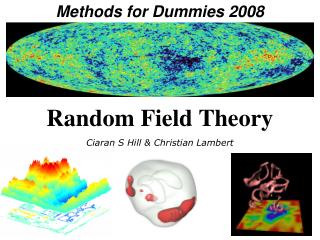
Random Field Theory
Random Field Theory. Will Penny SPM short course, London, May 2005. David Carmichael MfD 2006. image data. parameter estimates. design matrix. kernel. General Linear Model model fitting statistic image. realignment & motion correction. Random Field Theory. smoothing. normalisation.

Random Field Theory
E N D
Presentation Transcript
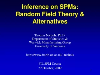
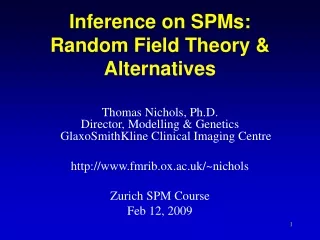
Random Field Theory Will Penny SPM short course, London, May 2005 David Carmichael MfD 2006
image data parameter estimates designmatrix kernel • General Linear Model • model fitting • statistic image realignment &motioncorrection Random Field Theory smoothing normalisation StatisticalParametric Map anatomicalreference corrected p-values
Overview 1. Terminology 2. Random Field Theory • Cluster level inference • SPM Results • FDR
Overview 1. Terminology • Random Field Theory • Cluster level inference • SPM Results • FDR
Inference at a single voxel NULL hypothesis, H: activation is zero a = p(t>u|H) p-value: probability of getting a value of t at least as extreme as u. If a is small we reject the null hypothesis. u=2 t-distribution u=(effect size)/std(effect size)
Sensitivity and Specificity ACTION Don’t Reject Reject H True TN FP H False FN TP TRUTH Specificity = TN/(# H True) = TN/(TN+FP) = 1 - a Sensitivity = TP/(# H False) = TP/(TP+FN) = b = power a = FP/(# H True) = FP/(TN+FP) = p-value/FP rate/sig level
Sensitivity and Specificity ACTION At u1 Don’t Reject Reject Spec=7/10=70% Sens=10/10=100% H True (o) TN=7 FP=3 H False (x) FN=0 TP=10 TRUTH Specificity = TN/(# H True) Sensitivity = TP/(# H False) Eg. t-scores from regions that truly do and do not activate o o o o o o o x x x o o x x x o x x x x u1
Sensitivity and Specificity ACTION Don’t Reject Reject At u2 H True (o) TN=9 FP=1 H False (x) FN=3 TP=7 TRUTH Spec=9/10=90% Sens=7/10=70% Specificity = TN/(# H True) Sensitivity = TP/(# H False) Eg. t-scores from regions that truly do and do not activate o o o o o o o x x x o o x x x o x x x x u2
Inference at a single voxel NULL hypothesis, H: activation is zero a = p(t>u|H) We can choose u to ensure a voxel-wise significance level of a. This is called an ‘uncorrected’ p-value, for reasons we’ll see later. We can then plot a map of above threshold voxels. u=2 t-distribution
Signal Inference for Images Noise Signal+Noise
Use of ‘uncorrected’ p-value, a=0.1 11.3% 11.3% 12.5% 10.8% 11.5% 10.0% 10.7% 11.2% 10.2% 9.5% Percentage of Null Pixels that are False Positives Using an ‘uncorrected’ p-value of 0.1 will lead us to conclude on average that 10% of voxels are active when they are not. This is clearly undesirable. To correct for this we can define a null hypothesis for images of statistics.
FAMILY-WISE NULL HYPOTHESIS: Activation is zero everywhere If we reject a voxel null hypothesis at any voxel, we reject the family-wise Null hypothesis A FP anywhere in the image gives a Family Wise Error (FWE) Family-wise Null Hypothesis Family-Wise Error (FWE) rate = ‘corrected’ p-value
Use of ‘uncorrected’ p-value, a=0.1 Use of ‘corrected’ p-value, a=0.1 FWE
The Bonferroni correction The Family-Wise Error rate (FWE), a, fora family of N independent voxels is α = Nv where v is the voxel-wise error rate. Therefore, to ensure a particular FWE set v = α / N BUT ...
The Bonferroni correction Assume Independent Voxels
Independent voxels - a good assumption?? • Voxel Point Spread Function (PSF) • - continuous signal is sampled for a discrete period • - imposes a filter that when FT’d gives a PSF • - Gives spread of signal through the image from point source • ..worse in PET • Physiological noise • Smoothing • Normalisation
The Bonferroni correction Independent Voxels Spatially Correlated Voxels Bonferroni is too conservative for brain images
Consider a statistic image as a discretisation of a continuous underlying random field Use results from continuous random field theory Random Field Theory Discretisation
Overview 1. Terminology • Random Field Theory • Cluster level inference • SPM Results • FDR
Topological measure threshold an image at u EC=# blobs at high u: Prob blob = avg (EC) So FWE, a = avg (EC) Euler Characteristic (EC)
Example – 2D Gaussian images • α = R (4 ln 2) (2π) -3/2 u exp (-u2/2) Voxel-wise threshold, u Number of Resolution Elements (RESELS), R N=100x100 voxels, Smoothness FWHM=10, gives R=10x10=100
Example – 2D Gaussian images • α = R (4 ln 2) (2π) -3/2 u exp (-u2/2) For R=100 and α=0.05 RFT gives u=3.8
How do we know number of resels? • We can simply use the FWHM of the smoothing kernel But processes such as normalisation mean smoothness will vary 2. Estimate the FWHM at each voxel using residuals at each voxel (worsley 1998)
volume Surface area diameter Euler # of space Resel Counts for Brain Structures (1) Threshold depends on Search Volume (2) Surface area makes a large contribution FWHM=20mm
Overview 1. Terminology 2. Theory 3. Imaging Data 4. Levels of Inference 5. SPM Results
Smoothness smoothness » voxel size practically FWHM 3 VoxDim Typical applied smoothing: Single Subj fMRI: 6mm PET: 12mm Multi Subj fMRI: 8-12mm PET: 16mm Applied Smoothing
Overview 1. Terminology 2. Theory 3. Imaging Data 4. Levels of Inference 5. SPM Results
Cluster Level Inference • We can increase sensitivity by trading off anatomical specificity • Given a voxel level threshold u, we can compute the likelihood (under the null hypothesis) of getting a cluster containing at least n voxels CLUSTER-LEVEL INFERENCE • Similarly, we can compute the likelihood of getting c clusters each having at least n voxels SET-LEVEL INFERENCE
n=12 n=82 n=32 Levels of inference voxel-level P(c 1 | n > 0, t 4.37) = 0.048 (corrected) At least one cluster with unspecified number of voxels above threshold set-level P(c 3 | n 12, u 3.09) = 0.019 At least 3 clusters above threshold cluster-level P(c 1 | n 82, t 3.09) = 0.029 (corrected) At least one cluster with at least 82 voxels above threshold
Overview 1. Terminology 2. Theory 3. Imaging Data 4. Levels of Inference 5. SPM Results
SPM results I Activations Significant at Cluster level But not at Voxel Level
SPM results II Activations Significant at Voxel and Cluster level
False Discovery Rate ACTION At u1 Don’t Reject Reject FDR=3/13=23% a=3/10=30% H True (o) TN=7 FP=3 H False (x) FN=0 TP=10 TRUTH Eg. t-scores from regions that truly do and do not activate FDR = FP/(# Reject) a = FP/(# H True) o o o o o o o x x x o o x x x o x x x x u1
False Discovery Rate ACTION Don’t Reject Reject H True (o) TN=9 FP=1 H False (x) FN=3 TP=7 TRUTH At u2 FDR=1/8=13% a=1/10=10% Eg. t-scores from regions that truly do and do not activate FDR = FP/(# Reject) a = FP/(# H True) o o o o o o o x x x o o x x x o x x x x u2
Signal False Discovery Rate Noise Signal+Noise
Control of Familywise Error Rate at 10% FWE Occurrence of Familywise Error Control of False Discovery Rate at 10% 6.7% 10.5% 12.2% 8.7% 10.4% 14.9% 9.3% 16.2% 13.8% 14.0% Percentage of Activated Pixels that are False Positives
Summary • We should not use uncorrected p-values • We can use Random Field Theory (RFT) to ‘correct’ p-values • RFT requires FWHM > 3 voxels • We only need to correct for the volume of interest • Cluster-level inference • False Discovery Rate is a viable alternative
Functional Imaging Data • The Random Fields are the component fields, Y = Xw +E, e=E/σ • We can only estimate the component fields, using estimates of w and σ • To apply RFT we need the RESEL count which requires smoothness estimates
^ Estimated component fields voxels ? ? = + parameters design matrix errors data matrix scans parameterestimates • estimate residuals estimated variance = Each row is an estimated component field estimatedcomponentfields