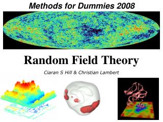
Methods for Dummies Random Field Theory
Methods for Dummies Random Field Theory. Annika Lübbert & Marian Schneider . Neural Correlates of Interspecies Perspective Taking in the Post-Mortem Atlantic Salmon. task > rest contrast. Bennett et al., (2010) in Journal of Serendipitous and Unexpected Results.

Methods for Dummies Random Field Theory
E N D
Presentation Transcript
Methods for Dummies Random Field Theory Annika Lübbert & Marian Schneider
Neural Correlates of Interspecies Perspective Taking in the Post-Mortem Atlantic Salmon task > rest contrast Bennett et al., (2010) in Journal of Serendipitous and Unexpected Results
Overview of Presentation 1. Multiple Comparisons Problem2. Classical Approach to MCP 3. Random Field Theory4. Implementation in SPM
Null Distribution of T Hypothesis Testing • To test an hypothesis, we construct “test statistics” and ask how likely that our statistic could have come about by chance • The Null Hypothesis H0 Typically what we want to disprove (no effect). The Alternative Hypothesis HA expresses outcome of interest. • The Test Statistic T The test statistic summarises evidence about H0. Typically, test statistic is small in magnitude when the hypothesis H0 is true and large when false. We need to know the distribution of T under the null hypothesis
1. Multiple Comparisons Problem u • Mass univariate analysis : perform t-tests for each voxel • test t-statistic against the null hypothesis -> estimate how likely it is that our statistic could • have come about by chance • Decision rule (threshold) u, • determines false positive rate • Choose u to give acceptableα • = P(type I error) i.e. chance we are wrong when rejecting the null hypothesis t = p(t>u|H)
1. Multiple Comparisons Problem u u u u u • Problem: fMRI – lots of voxels, lots of t-tests • If use same threshold, inflated probability of obtaining false positives t t t t t
t > 2.5 t > 4.5 t > 0.5 t > 1.5 t > 3.5 t > 5.5 t > 6.5 Example • T-map for whole brain may contain say • 60000 voxels • Each analysed separately would mean • 60000 t-tests • At = 0.05 this would be 3000 false positives (Type 1 Errors) • Adjust threshold so that any values above threshold are unlikely to under the null hypothesis (height thresholding& take into account the number of tests.) t > 0.5
Neural Correlates of Interspecies Perspective Taking in the Post-Mortem Atlantic Salmon task > rest contrast t(131) > 3.15, p(uncorrected) < 0.001, resulting in 3 false positives
Bonferroni Correction = PFWE / n α= new single-voxel threshold n = number of tests (i.e. Voxels) FWE = family-wise error
Bonferroni Correction Example single-voxel probability threshold Number of voxels • = PFWE / n • e.g. 100,000 t stats, all with 40 d.f. • For PFWE of 0.05: • 0.05/100000 = 0.0000005 , • corresponding t=5.77 • => a voxel statistic of t>5.77 has only a 5% chance of arising anywhere in a volume of 100,000 t stats drawn from the null distribution Family-wise error rate
Why Bonferroni is too conservative • Functional imaging data has a degree of spatial correlation • Number of independent values < number of voxels • Why? • The way that the scanner collects and reconstructs the image • Physiology • Spatial preprocessing (resampling, smoothing) • Fundamental problem: image data represent situation in which we have a continuous statistic image, not a series of independent tests
Illustration Spatial Correlation Single slice image with 100 by 100 voxels Filling the voxel values with independent random numbers from the normal distribution Bonferroni accurate
Illustration Spatial Correlation add spatial correlation: break up the image into squares of 10 by 10 pixels calculate the mean of the 100 values contained 10000 numbers in image but only 100 independent Bonferroni 100 times too conservative!
Smoothing contributes Spatial Correlation • Smooth image by applying a Gaussian kernel with FWHM = 10 (at 5 pixels from centre, value is half peak value) • Smoothing replaces each value in the image with weighted average of itself and neighbours • Blurs the image -> reduces number of independent observations
Smoothing Kernel FWHM (Full Width at Half Maximum)
Using RFT to solve the Multiple Comparison Problem (get FWE) • RFT approach treats SPMs as a discretisation of underlying continuous fields • Random fields have specified topological characteristics • Apply topological inference to detect activations in SPMs
Three stages of applying RFT: 1. Estimate smoothness 2. Find number of ‘resels’ (resolution elements) 3. Get an estimate of the Euler Characteristic at different thresholds
1. Estimate Smoothness • Given: Image with applied and intrinsic smoothness • Estimated using the residuals (error) from GLM Estimate the increase in spatial correlation from i.i.d. noise to imaging data (‘from right to left’) estimate
2. Calculate the number of resels • Look at your estimated smoothness(FWHM) • Express your search volume in resels • Resolution element (Ri = FWHMx x FWHMy x FWHMz) • # depends on smoothness of data (+volume of ROI) • “Restores” independence of the data
3. Get an estimate of the Euler Characteristic • Steps 1 and 2 yield a ‘fitted random field’ (appropriate smoothness) • Now: how likely is it to observe above threshold (‘significantly different’) local maxima (or clusters, sets)under H0? • How to find out? EC!
Euler Characteristic – a topological property • Leonhard Euler 18th century swiss mathematician • SPM threshold EC • EC = number of blobs (minus number of holes)* “Seven bridges of Kӧnisberg” *Not relevant: we are only interested in EC at high thresholds (when it approximates P of FEW)
Euler Characteristic and FWE Zt = 2.5 EC = 3 • The probability of a family wise error is approximately equivalent to the expected Euler Characteristic • Number of “above threshold blobs” Zt = 2.75 EC = 1
How to get E [EC] at different thresholds # of resels Expected Euler Characteristic Z (or T) -score threshold * Or Monte Carlo Simulation, but the formula is good! It gives exactestimates, as long as your smoothness is appropriate
Given # of resels and E[EC], we can find the appropriate z/t-threshold E [EC] for an image of 100 resels, for Z score thresholds 0 – 5
How to get E [EC] at different thresholds # of resels Expected Euler Characteristic Z (or T) -score threshold From this equation, it looks like the threshold depends only on the number of reselsin our image
Shape of search region matters, too! • #resels E [EC] • not strictly accurate! • close approximation if ROI is large compared to the size of a resel • #+ shape + size resel • E [EC] • Matters if small or oddly shaped ROI • Example: • central 30x30 pixel box = max. 16 ‘resels’ (resel-width = 10pixel) • edge 2.5 pixel frame = same volume but max. 32 ‘resels’ • Multiple comparison correction for frame must be more stringent
Different types of topological Inference • localizing power! • …intermediate… • sensitivity! intensity • Topological inference can be about • Peak height (voxel level) • Regional extent (cluster level) • Number of clusters (set level) t Different height and spatial extent thresholds tclus space
Assumptions made by RFT • Underlying fields are continuous with twice-differentiable autocorrelation function • Error fields are reasonable lattice approximation to underlying random field with multivariate Gaussian distribution lattice representation • Check: FWHM must be min. 3 voxels in each dimension • In general: if smooth enough + GLM correct (error = Gaussian) RFT
Assumptions are not met if... • Data is not sufficiently smooth • Small number of subjects • High-resolution data • Non-parametric methods to get FWE (permutation) • Alternative ways of controlling for errors: FDR (false discovery rate)
Take-home message, overview: Large volume of imaging data Multiple comparison problem <smoothing with a Gaussian kernel, FWHM > Mass univariate analysis Uncorrected p value Too many false positives Bonferroni correction α=PFWE/n Corrected p value Random field theory (RFT) α=PFWE ≒ E[EC] Corrected p value Null hypothesis rarely rejected Too many false negatives Never use this.
Thank you for your attention! …and special thanks to Guillaume!
Sources • Human Brain Function, Chapter 14, An Introduction to Random Field Theory (Brett, Penny, Kiebel) • http://www.fil.ion.ucl.ac.uk/spm/course/video/#RFT • http://www.fil.ion.ucl.ac.uk/spm/course/video/#MEEG_MCP • Former MfD Presentations • Expert Guillaume Flandin