Infilling Radar CAPPIs
390 likes | 411 Vues
Explore the methodology behind infilling radar CAPPI data for accurate rainfall estimation at ground level. Learn about strategies to correct bright band effects and optimize rainfall classification algorithms for better results.

Infilling Radar CAPPIs
E N D
Presentation Transcript
Infilling Radar CAPPIs Geoff Pegram, Scott Sinclair, Stephen Wesson & Pieter Visser
What we’ve done … • We can remove ground-clutter and have improved the estimation of rainfall by radar at ground level • We have refined the merged fields of radar with raingauge data • We think that the combined fields are good out to 75 km from the radar with a reasonably dense network of gauges, but we’re happy to take advice!
NATIONAL WEATHER RADAR NETWORKsee Deon’s presentation Existing radars Radars added (2004) Planned radars
Ground clutter contamination can be extensive Results in poor quality rainfall estimates Parts of radar volume scan where data is unknown Rainfall estimates at ground level unknown Problems with Radar CAPPI Data
Summary of Infilling Strategy • Choose Rainfall classification algorithm • Devise Bright band correction algorithm • Semivariogram parameters determined by rainfall type. Climatological semivariograms. • Ordinary and Universal Kriging to extrapolate rain information. Universal Kriging utilised in mixed zone. • Cascade Kriging to progressively infill data down to ground.
Rainfall Classification • Rainfall separated into two zones: (1) Convective Zone (2) Stratiform Zone • Criteria of classification set out in table below.
Classified Images X X 18 km dBZ 0 km CROSS SECTION X-X 18 km Classification 0 km Examples of Rainfall Classification Reflectivity Images
Characteristicsof Classified Rainfall • Stratiform – low average height, low variability and intensity. • Convective –considerable vertical extent, high variability and intensity. • Increase of rainfall intensity nearer ground level
Climatological Profile Affected by Bright Band with Extrapolation to Ground Level Corrected Climatological Profile Typical Climatologial Profile Rainfall Estimate at Ground Level New Rainfall Estimate at Ground Level Climatological Profile Affected by Bright Band Climatological Profile Correction Procedure CAPPI level affected by bright band CAPPI level affected by bright band corrected BrightBandCorrection • Bright Band – melting snow & ice crystals • Need to correct bright band to obtain accurate rainfall estimates at ground level • Proposed correction procedure: pixel by pixel approach Height (km) 4 km 3 km 2 km 1 km Reflectivity (dBZ)
2km CAPPI pixels marked which are affected by bright band 2km CAPPI after bright band correction 2km CAPPI before bright band correction BrightBandCorrection • Testing of bright band correction • Results: improved rainfall estimates at ground level
30km SILL RANGE Semivariogram Modeling • Semivariogram model parameters computed for convective & stratiform rain in horizontal & vertical directions Reflectivity Image
Graphs indicating clustering of alpha and correlation length parameters by rainfall type (15 Rain Events over 4 different years) Table of Average Parameters:
Convective Cluster: Lc , c Stratiform Cluster: Ls , s L, α + σα L, α - σα L - σL, α L, α L + σL, α L, α + σα L, α - σα L - σL, α L, α L + σL, α Sensitivity Analysis of Stratiform, Horizontal Parameters Missing data infilled with different combinations of α and L that represent the spread of parameter values. No significant difference between Kriging estimates returned for spread of parameter values
KRIGING used to extrapolate/interpolate horizontal and vertical rainfall information to infill unknown data points Considered to be the optimal technique for interpolation of Gaussian data Computational Efficiency & Stability: Nearest 25 rainfall values used in Kriging Singular Value Decomposition (SVD) with trimming of small singular values to ensure computational stability Kriging to Infill Missing Rain Data
stratiform pixel • convective pixel • target pixel Summary: Three Rainfall Zones Stratiform Zone All controls stratiform. OK used to infill target point. Convective Zone All controls convective. OK used to infill target point. Mixed Zone Controls stratiform & convective. UK used to infill target point.
Rainrate (mm/hr) Reflectivity (dBZ) Rainrate (mm/hr) Reflectivity (dBZ) RAINRATE ERROR MAPS Absolute Error 0 50 100 All Errors Rainrate (mm/hr) Reflectivity (dBZ) & |Rainrate Errors| (mm/hr) Mixed Rainrate Errors (mm/hr) Stratiform Rainrate Errors (mm/hr) Convective Rainrate Errors (mm/hr) Validation: Universal & Ordinary Kriging Kriging Estimate Observed Rainfall
UK & OK Effectiveness • UK & OK tested on three different rainfall zones on a variety of instantaneous images • Effectiveness evaluated by comparing mean, and Σdifference2of estimated & observed rainfall • UK in mixed zone provides a superior estimate than OK and reduced Σdifference2
Inflation of Kriged values Discontinuities 80 20 40 0 60 100 Rainfall Accumulation (mm) KRIGING directly to Ground Level • Unexpected problems with CAPPI edges • Higher Kriged values returned than expected and serious discontinuity also evident • Example: 24 hour accumulation
3D CASCADE KRIGING EXAMPLE Radar Volume Scan Data Radar Volume Scan Data After Cascade Kriging
Ground Clutter contaminates radar volume scan data up to 5km above ground level. Ground Clutter 3km above ground level Ground Clutter infilled on 3km level Reflectivity estimation at ground level CASCADE KRIGING: Ground Clutter
Ground clutter segments to be estimated Ground Clutter Map Superimposed Original Reflectivity Image Estimated reflectivity data Convert to rain rate by Marshall-Palmer equation Store estimated and observed rain rate values and proceed to next image in sequence Testing: Ground Clutter Infilling • Tested on 3D Bethlehem ground clutter map • Ground clutter placed onto known rain • Tested on three different rain events over 24hr period
Results: Ground Clutter Infilling • Accumulations over 6, 12 and 24 hours show close correspondence between observed and estimated values
Liebenbergsvlei Catchment Raingauge Locations MRL5 Weather Radar Bethlehem 1 km 1 km Radar Pixel Locations Rainguage Locations 2 L Selection Range Testing: Rainfall Estimation at Ground Level Polokwane • Extrapolated radar estimates at ground level compared to raingauge estimates Irene Ermelo Bloemfontein Bethlehem De Aar Durban East London Port Elizabeth Cape Town
Results: Rainfall Estimation at Ground Level • Two rain events selected of different rainfall types – 12h & 24 h accumulations • Results indicate fair estimation of rainfall at ground level • We’ve got a handle on the errors
The Conditional Merging algorithm To combine radar and gauge data optimally: • Krige the gauges to give best guess field, MG • Krige the radar pixels at gauge locations, MR • If RR is the measured radar rainfield, • Conditional Merged Field is: RC = RR + MG – MRwhich coincides with the gauges and interpolates intelligently
A real cross-validation field experiment • Compare straight Kriging and Conditional Merging on 45 rain gauges on a 4600 km2 catchment • Use cross-validation – estimation of daily total at each gauge separately using the remaining data
Errors with range – how good is the radar? • 22 new gauges • 4 different days of accums
Concluding Remarks • With intelligent extrapolation and climatoloical variograms we can get good ground estimates • With conditional merging of radar and gauge data we can get good interpolation to adjust for errors in the Z-R formula • Within 75 km from the radars, we can offer sound areas in varying climates and land cover in our expanding radar and gauge network